DSP Builder for Intel® FPGAs (Advanced Blockset): Handbook
A newer version of this document is available. Customers should click here to go to the newest version.
14.4.20. CORDIC
The CORDIC algorithm is a simple and efficient algorithm that calculates:
- Vector rotations
- Trigonometric functions such as sine and cosine
- Inverse trigonometric functions such as the arctangent
- Vector magnitudes
The CORDIC block can calculate all these functions. However, it does not calculate hyperbolic functions, square roots, logarithms and exponentials.
Generally, the CORDIC block is faster than other approaches in the absence of hardware multipliers or when multipliers become a scarce resource in your design. For low precision designs, you can also consider implementations based on direct table lookups.
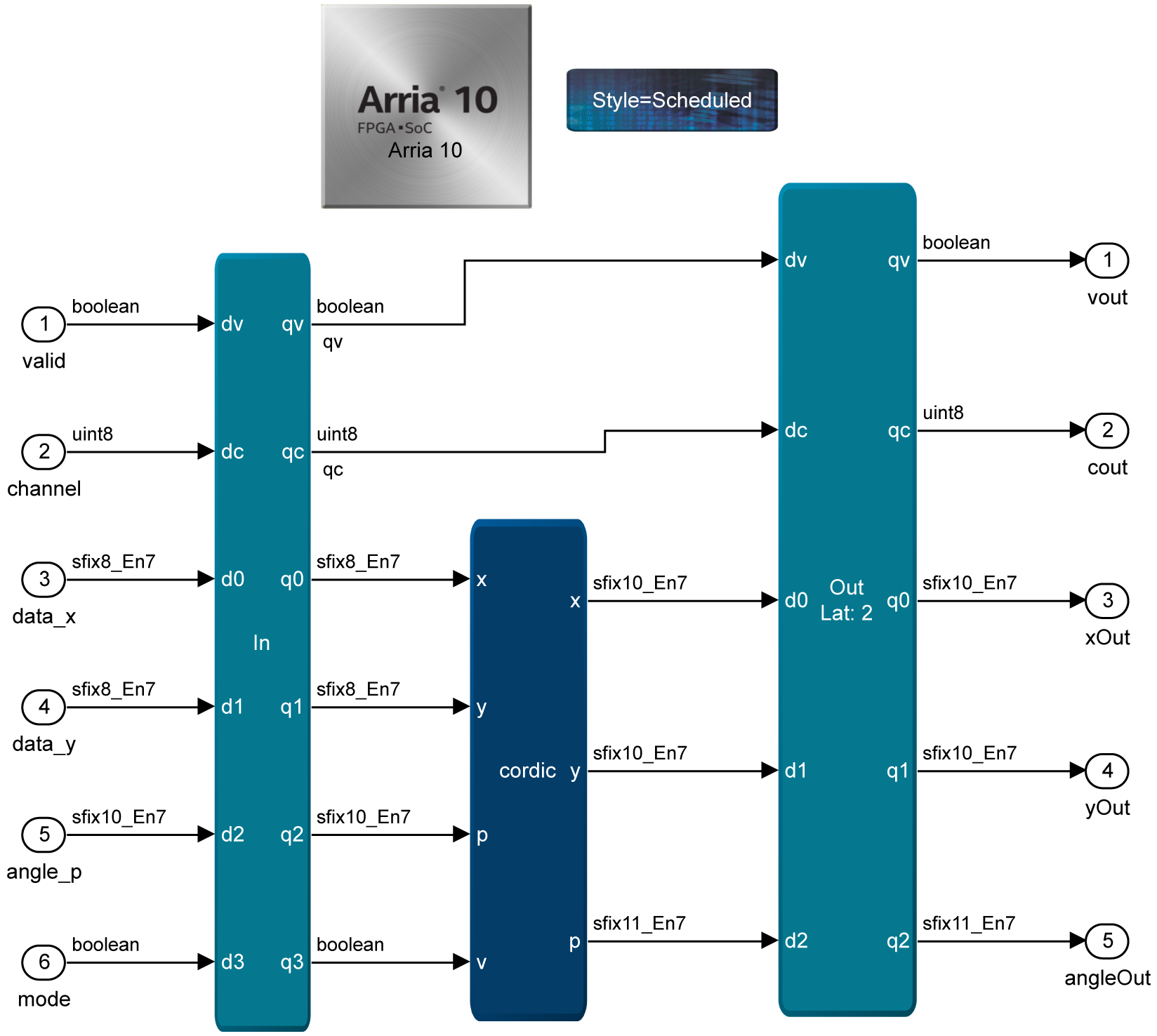
The CORDIC block takes four inputs x, y, p and v. The x and y inputs provide the cartesian coordinates (x, y) of an input vector. The p input provides an input angle. Input v allows run-time switching between the two modes of the CORDIC block. The block has three outputs denoted by the same x, y, and p.
You can configure the CORDIC block at runtime to change between rotation and vector modes. Rotation mode allows rotating a vector defined by its cartesian coordinates by an angle provided in radians. By providing specific input vector coordinates, rotation mode also allows computing the sine and cosine of the input angle. The vector mode inputs a vector and rotates the vector until its y component is zero, and its x component is positive. The mode allows computing the arctangent of the input angle in radians and the magnitude of the input vector.
The generic CORDIC iterations are:
The computation of s[i] depends on the mode:
| Rotation Mode | s[i] = +1 if p[i] ≥ 0, otherwise –1 |
| Vector Mode | s[i] = +1 if y[i] < 0, otherwise –1 |
In rotation mode, active when input v is 0, the CORDIC rotates the input vector by a specified angle. The input vector is defined by its cartesian coordinates provided on the x and y inputs. You provide the angle by which this vector is rotated on input p. The angle must have a value in the interval. You read the output vector coordinates from the x and y outputs of the block. The block does not use output p in this mode. The output equations for this mode are:
The equation also shows how you can obtain the sine and cosine of the input angle p.
Setting and gives:
In vector mode, active when the input v is 1, the CORDIC block rotates the input vector to the x-axis and records the angle required to make that rotation. The same as for rotation mode, you provide the input vector coordinates on the x and y inputs. Initialize the input p with the value 0. The output p contains the angle that the input vector v makes with the positive x-axis. This angle is in the interval .The first output x saves the magnitude of the input vector v.
The output equations of both the rotation and vector modes show that K(n) multiplies either the coordinates of the resulting output vector, or the magnitude of the vector. K(n) is a CORDIC-specific scale factor (also referred to as gain) that amplifies the outputs. You can statically compute the gain for a known number of iterations of the algorithm. You can compensate for the gain effects, external to the CORDIC block, by using a constant multiplication by 1/K(n).
You can calculate the gain K(n) incrementally as the product of individual gains per step. The step gain denoted by K i is :
where i represents the iteration index, starting from 0.
The total gain is the product of the step gains K i . Therefore, for n iterations of the CORDIC algorithm the gain is equal to:
The CORDIC gain is not automatically compensated in the CORDIC block. Using w as the width in bits of the x and y inputs (their widths and formats needs to match), the width of the x and y outputs is by default set to w+2, where the 2 additional bits are added in the MSB position. The additional bits allow accounting for the gain factor without overflow.
The p input is the angular value and has a range between and , which requires three integer bits to fully represent the range. The CORDIC block requires that the format of the signal feeding into the p input has exactly three integer bits, and that it is signed. Denoting by q the width in bits of the input p, the width of the output p is q+1. The additional bit is added in the MSB position. It allows for subtracting an angle provided on the input p from the computed arctangent of the input vector (when the block is in vectoring mode) without overflowing.
| Parameter | Description |
|---|---|
| Output data type mode | Determines how the block sets its output data type:
|
| Output data type | Specifies the output data type. For example, sfix(16), uint(8). |
| Output scaling value | Specifies the output scaling value. For example, 2^-15. |
| Signal | Direction | Type | Description | Vector Data Support | Complex Data Support |
|---|---|---|---|---|---|
| x | Input | Signed fixed-point type | x coordinate of the input vector. | Yes | Yes |
| y | Input | Signed fixed-point type | y coordinate of the input vector. | Yes | Yes |
| p | Input | Signed type with three integer bits. | Required angle of rotation in the range between –pi and +pi. | Yes | Yes |
| v | Input | Unsigned 1-bit wide integer or Boolean. | Selects the mode of operation 0 = rotation mode, 1 = vector mode.. | Yes | Yes |
| x | Output | When the output data type mode is set to inherit via internal rule, the type of the output port x is the same as the input port x, with the same alignment but two additional bits to cope with the gain. | x coordinate of the output vector. | Yes | Yes |
| y | Output | When the output data type mode is set to inherit via internal rule, the type of the output port x is the same as the input port x, with the same alignment but two additional bits to cope with the gain. | y coordinate of the output vector. | Yes | Yes |
| p | Output | Same alignment as the input port p, with one additional MSB. | In vector mode (v=1), it returns the angle of input vector defined by its cartesian coordinates x and y. The returned angle is in the interval [-pi, pi]. | Yes | Yes |
Numeric Example
This complete numeric example for both modes of the CORDIC block uses this configuration:
- Input data types for the x and y inputs are sfix8_en7 (corresponding to a w = 8-bit wide signed format having 7 fractional bits)
- The input type for input p is sfix10_en7 (corresponding to a q=10-bit wide signed format having 7 fractional bits).
Whenever the example uses binary representation of values, it suffixes the values by _2 to distinguish them from base 10 values.
Rotation Mode Example
To depict the functioning of the block in rotation mode, set the inputs of the block to:
Table 189 shows the operation of the CORDIC block in rotation mode, in which the (x,y) vector is rotated by the angle p. The first column shows the iteration index. The CORDIC block inputs w=8-bit signals and performs 10 iterations internally. At each iteration, the signals x[i], y[i] and p[i] are updated based on the values x[i-1], y[i-1] and p[i-1] computed by the previous iteration.
For each iteration, the first row shows the equations for computing the values, for instance:
y[4] = y[3] + s[3]*2^(-3)x[3])
Whereas the second row shows the actual value computed, in both binary and decimal representation (001.1010010_2 (1.640625)). The binary representation uses the 2’s complement notation. The rightmost column shows the formula to compute the corresponding step-gain and the gain-step value, in decimal.
| Iter. | x | y | p | s | k i |
|---|---|---|---|---|---|
| init. | x[0]= 0.1100000_2 (0.75) | y[0]= 0.1100000_2 [0.75] | p[0]=0.1000011_2 [0.5234375] | s[0]=+1 | |
| 1 | x[1]=x[0]-s[0](2^-0)y[0] | y[1] = y[0] + s[0](2^-0)x[0] | p[1] = p[0] - s[0]atan(2^-0) | k 0 = sqrt(1 + 2-2×0) | |
| 000.0000000_2 (0.0) | 001.1000000_2; (1.5) | 111.1011110_2; (-0.265625) | s[1]=-1 | k 0 ≈ 1.4142 | |
| 2 | x[2] = x[1] - s[1]2^(-1)y[1] | y[2]=y[1] + s[1]2^(-1)x[1] | p[2] = p[1] - s[1]atan(2^-1) | k 1 = sqrt(1 + 2-2×1) | |
| 000.1100000_2 (0.75) | 001.1000000_2 (1.5) | 000.0011001_2; (0.1953125) | s[2]=+1 | k 1 ≈ 1.11803 | |
| 3 | x[3] = x[2] - s[2]2^(-2)y[2] | y[3] = y[2] + s[2]2^(-2)x[2] | p[3] = p[2] - s[2]atan(2^-2) | k 2 = sqrt(1 + 2-2×2) | |
| 000.0110000_2 (0.375) | 001.1011000_2 (1.6875) | 111.1111010_2;(-4.6875e-2) | s[3]=-1 | k 2 ≈ 1.030776 | |
| 4 | x[4] = x[3] - s[3]2^(-3)y[3] | y[4] = y[3] + s[3]2^(-3)x[3] | p[4] = p[3] - s[3]atan(2^-3) | k 3 = sqrt(1 + 2-2×3) | |
| 000.1001011_2 (0.5859375) | 001.1010010_2 (1.640625) | 000.0001010_2 (7.8125e-2) | s[4]=+1 | k 3 ≈ 1.0077822 | |
| 5 | x[5] = x[4] - s[4]2^(-4)y[4] | y[5] = y[4] + s[4]2^(-4)x[4] | p[5] = p[4] - s[4]atan(2^-4) | k 4 = sqrt(1 + 2-2×4) | |
| 000.0111110_2 (0.484375) | 001.1010110_2 (1.671875) | 000.0000010_2 (1.5625e-2) | s[5]=+1 | k 4 ≈ 1.001951 | |
| 6 | x[6] = x[5] - s[5]2^(-5)y[5] | y[6] = y[5] + s[5]2^(-5)x[5] | p[6] = p[5] - s[5]atan(2^-5) | k 5 = sqrt(1 + 2-2×5) | |
| 000.0111000_2 (0.4375) | 001.1010111_2 (1.6796875) | 111.1111110_2 (-1.5625e-2) | s[6]=-1 | k 5 ≈ 1.000488 | |
| 7 | x[7] = x[6] - s[6]2^(-6)y[6] | y[7] = y[6] + s[6]2^(-6)x[6] | p[7] = p[6] - s[6]atan(2^-6) | k 6 = sqrt(1 + 2-2×6) | |
| 000.0111011_2 (0.4609375) | 1.1010111_2 (1.6796875) | 000.0000000_2; (0.0) | s[7]=+1 | k 6 ≈ 1.000122 | |
| 8 | x[8] = x[7] - s[7]2^(-7)y[7] | y[8] = y[7] + s[7]2^(-7)x[7] | p[8] = p[7] - s[7]atan(2^-7) | k 7 = sqrt(1 + 2-2×7) | |
| 000.0111010_2 (0.453125) | 1.1010111_2 (1.6796875) | 111.1111111_2; (-7.8125e-3) | s[8]=-1 | k 7 ≈ 1.000030 | |
| 9 | x[9] = x[8] - s[8]2^(-8)y[8] | y[9] = y[8] + s[8]2^(-8)x[8] | p[9] = p[8] - s[8]atan(2^-8) | k 8 = sqrt(1 + 2-2×8) | |
| 000.0111010_2; (0.453125) | 1.1010111_2 (1.6796875) | 111.1111111_2; (-7.8125e-3) | s[9]=-1 | k 8 ≈ 1.000007 | |
| 10 | x[10] = x[9] - s[9]2^(-9)y[9] | y[10] = y[9] + s[9]2^(-9)x[9] | p[10] = p[9] - s[9]atan(2^-9) | k 9 = sqrt(1 + 2-2×9) | |
| 000.0111010_2; (0.453125) | 1.1010111_2 (1.6796875) | 111.1111111_2; (-7.8125e-3) | k 9 ≈ 1.000001 |
The CORDIC gain after 10 iterations is K(n)=K(w+2) = K(10)
Accuracy of the Rotate Mode Example
The example achieves compensation for the gain by multiplying the output vector coordinate values by . Post compensation and after rounding to the 7-bit fraction, the output vector coordinates are:
The absolute error for each coordinate is:
The unit in the last place (ULP) of the output format is 2-7, which makes the 2-10 output error particularly small for this set of inputs.
- The input vector (x(0), y(0)) is rotated to (x(1), y(1)) by atan(1)=pi/4.
- The vector is rotated back by atan(1/2) to (x(2),y(2)).
- This vector is rotated forward by atan(1/4) to (x(3), y(3)).
- This vector is rotated back by atan(1/8) to (x(4), y(4)).
This process continues for ten iterations (for clarity the figure does not show all intermediary vectors). The figure shows in blue the resulting vector after ten iterations, (x(10), y(10)). It comes as a result of successive microrotations by angles corresponding to atan(2^(-i) ). The sign of the values in the “s” column in Table 189 gives the direction of each microrotation.
The figure also shows how the magnitude of the input vector increases with the iterations. The largest increase happens in the first three iterations (refer to the step gains K 0, K 1 and K 2 in Table 189).
Vector Mode Example
For this example, the inputs are:
| Iter. | x | y | p | s | k i |
|---|---|---|---|---|---|
| Init | x[0]=0.1100000_2 (0.75) | 0.1100000_2 (0.75) | p[0] = 000.0000000_2 (0.0) | s[0]=-1 | |
| 1 | x[1] = x[0] - s[0](2^-0)y[0] | y[1] = y[0] + s[0](2^-0)x[0] | p[0] - s[0]atan(2^-0) | k 0 = sqrt(1 + 2-2×0) | |
| 001.1000000_2; (1.5) | 000.0000000_2; (0.0) | 000.1100101_2 (+0.7890625) | s[1]=-1 | k 0 ≈ 1.4142 | |
| 2 | x[2] = x[1] - s[1](2^-1)y[1] | y[2] = y[1] + s[1](2^-1)x[1] | p[1] - s[1]atan(2^-1) | k 1 = sqrt(1 + 2-2×1) | |
| 001.1000000_2; (1.5) | 111.0100000_2; (-0.75) | 001.0100000_2 (1.25) | s[2]=+1 | k 1 ≈ 1.11803 | |
| 3 | x[3] = x[2] - s[2](2^-2)y[2] | y[3] = y[2] + s[2](2^-2)x[2 | p[3] = p[2] - s[2]atan(2^-2 | k 2 = sqrt(1 + 2-2×2) | |
| 001.1011000_2; (1.6875) | 111.1010000_2; (-0.375) | 001.0000001_2; (1.0078125) | s[3]=+1 | k 2 ≈ 1.030776 | |
| 4 | x[4] = x[3] - s[3](2^-3)y[3] | y[4] = y[3] + s[3](2^-3)x[3] | p[4] = p[3] - s[3]atan(2^-3) | k 3 = sqrt(1 + 2-2×3) | |
| 001.1011110_2 (1.734375) | 111.1101011_2 (-0.1640625) | 000.1110001_2 (0.8828125) | s[4]=+1 | k 3 ≈ 1.0077822 | |
| 5 | x[5] = x[4] - s[4](2^-4)y[4] | y[5] = y[4] + s[4](2^-4)x[4] | p[5] = p[4] - s[4]atan(2^-4) | k 4 = sqrt(1 + 2-2×4) | |
| 001.1100000_2 (1.75) | 111.1111000_2 (-6.25e-2) | 000.1101001_2 (0.8203125) | s[5]=+1 | k 4 ≈ 1.001951 | |
| 6 | x[6] = x[5] - s[5](2^-5)y[5] | y[6] = y[5] + s[5](2^-5)x[5] | p[6] = p[5] - s[5]atan(2^-5) | k 5 = sqrt(1 + 2-2×5) | |
| 001.1100001_2 (1.7578125) | 111.1111111_2 (-7.8125e-3) | 000.1100101_2 (0.7890625) | s[6]=+1 | k 5 ≈ 1.000488 | |
| 7 | x[7] = x[6] - s[6](2^-6)y[6] | y[7] = y[6] + s[6](2^-6)x[6] | p[7] = p[6] - s[6]atan(2^-6) | k 6 = sqrt(1 + 2-2×6) | |
| 001.1100010_2 (1.765625) | 000.0000010_2 (1.5625e-2) | 000.1100011_2 (0.7734375) | s[7]=-1 | k 6 ≈ 1.000122 | |
| 8 | x[8] = x[7] - s[7](2^-7)y[7] | y[8] = y[7] + s[7](2^-7)x[7] | p[8] = p[7] - s[7]atan(2^-7) | k 7 = sqrt(1 + 2-2×7) | |
| 001.1100010_2 (1.765625) | 000.0000001_2 (7.8125e-3) | 000.1100100_2 (0.78125) | s[8]=-1 | k 7 ≈ 1.000030 | |
| 9 | x[9] = x[8] - s[8](2^-8)y[8] | y[9] = y[8] + s[8](2^-8)x[8] | p[9] = p[8] - s[8]atan(2^-8) | k 8 = sqrt(1 + 2-2×8) | |
| 001.1100010_2 (1.765625) | 000.0000001_2 (7.8125e-3) | 000.1100100_2 (0.78125) | s[9]=-1 | k 8 ≈ 1.000007 | |
| 10 | x[10] = x[9] - s[9](2^-9)y[9] | y[10] = y[9] + s[9](2^-9)x[9] | p[10] = p[9] - s[9]atan(2^-9) | k 9 = sqrt(1 + 2-2×9) | |
| 001.1100010_2 (1.765625) | 000.0000001_2 (7.8125e-3) | 000.1100100_2 (0.78125) | k 9 ≈ 1.000001 |
To obtain the magnitude of the input vector, divide the output on X[10] by K(10) to give:
When rounding to a 7-bit fraction format, the computed value, post scale factor compensation is:
The golden value corresponding to the vector magnitude is:
The absolute error on the vector magnitude is:
The vector magnitude error for this set of inputs is the same order of magnitude as the ULP value.
Compute the accuracy of the returned angle by subtracting it from the golden value, or pi/4:
Thus the relative error on the angle component for this set of inputs is roughly half ULP.