Software Optimization for Intel® GPUs (NEW)
Use Intel® VTune™ Profiler to estimate overhead when offloading onto an Intel GPU. Analyze the performance of computing tasks offloaded onto the GPU.
The increasing popularity of heterogeneous computing has led performance-conscious developers to discover that different types of workloads perform best on different hardware architectures. Intel provides many high-performance architectures including CPUs, GPUs, and FPGAs. This methodology describes how you use VTune Profiler to profile and optimize compute-intensive workloads offloaded onto Intel GPUs.
Understand Your Intel GPU
- Employ parallelism: Extracting superior performance from a workload-intensive GPU begins with an understanding of GPU architecture and functionality. A GPU employs a high level of parallelism with several smaller processing cores that work together. A GPU is well suited for workloads that can be split into tasks that run concurrently. Single-core serial performance on a GPU is much slower than on a CPU. Therefore, applications must take advantage of the massive parallelism available in a GPU.
- Move data intelligently: Using a GPU requires you to move data to and from the GPU, which can create overhead and impact performance. Marshall data intelligently to take advantage of temporal and spatial locality in the GPU. Using registers and caches to store data close together is important to get the best performance.
- Use the offload model: Although your GPU is available to handle the most significant parts of your workload, your CPU is still vital to perform other workload tasks. Use the GPU in an offload model, where you offload some portion of your workload onto the GPU(target) device. The GPU functions as an accelerator for those parts that perform best on the GPU. The CPU(host) executes the rest of the workload. Optimizing software performance in this context centers on two major tasks:
- Optimal offload onto a GPU
- Optimization for the GPU
- What to offload
- How to offload
- How to write the GPGPU algorithm
- How to use GPU Offload Analysis in VTune Profiler to analyze GPU offload performance
Intel GPU Architecture
Before we examine the GPU offload model, let us first examine the architecture of an Intel GPU, like the Gen9 GT2 GPU. This device is integrated into Intel® microarchitecture codenamed Skylake. You can program this GPU using high level languages like OpenCL* and SYCL*.
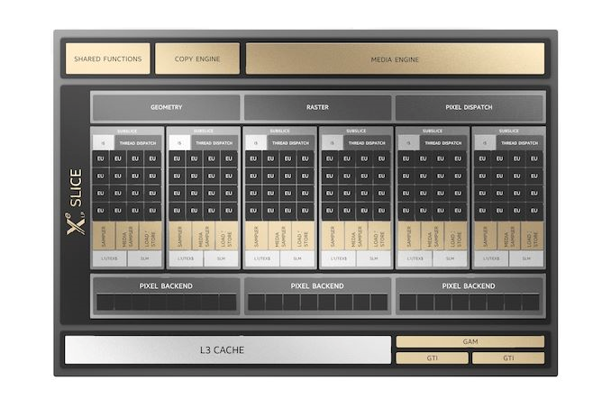
The Gen9 GT2 GPU has a single slice with 24 Execution Units (EUs). An Execution Unit is the foundational building block of GPU architecture.
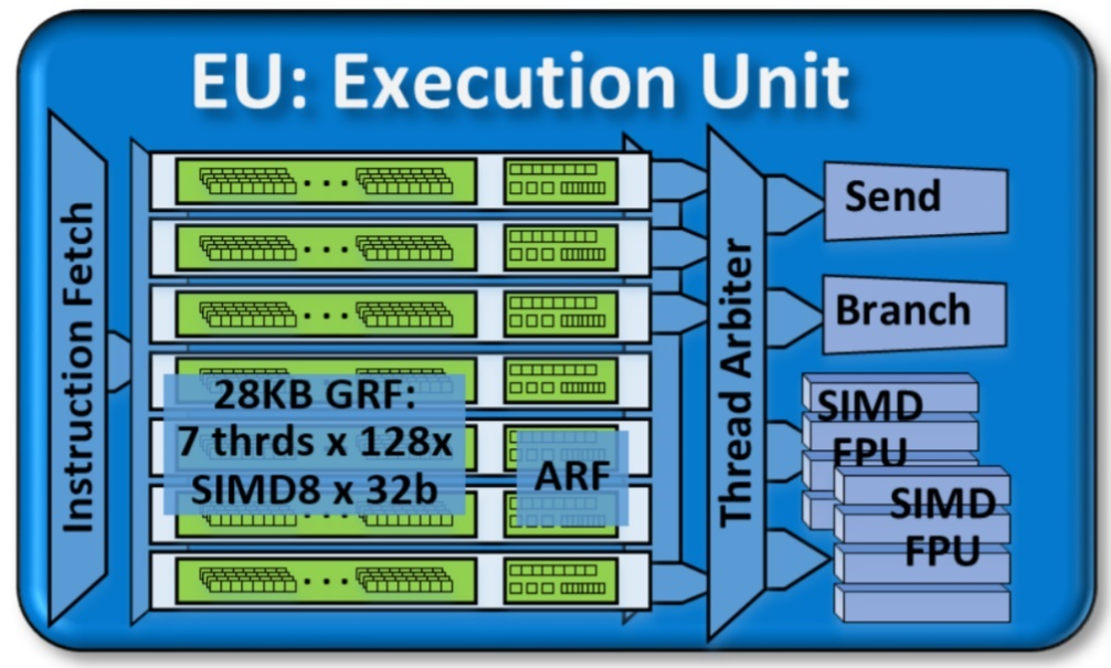
An EU is a combination of simultaneous multi-threading (SMT) and fine-grained interleaved multi-threading (IMT). EUs are computing processors that drive multiple issue, Single Instruction Multiple Data Arithmetic Logic Units (SIMD ALUs). These SIMD ALUs are pipelined across multiple threads. SIMD ALUs are useful for high-throughput floating-point and integer computations. The fine-grain threaded nature of the EUs ensures continuous streams of instructions that are ready for execution. The IMT also hides the latency of longer operations like memory scatter/gather, sampler requests, or other system communications.
The thread arbiter dispatches several instructions in each cycle of operation. When these instructions do not propagate to functional units, there is a stall. The duration of a stall is measured by the number of execution cycles that passed in that state. This measure helps us estimate the efficiency of EUs. The EU Array Stalled metric counts the number of cycles when the EU was stalled but at least a single thread was active. The stalling could happen when the EU was waiting for data from a memory subsystem. See GPU Metrics Reference (in the VTune Profiler User Guide) for more information on related GPU metrics.
To use the full computing power of a massively parallel machine, you must provide all EUs in the GPU with enough calculations to execute. Therefore, EUs have more hardware threads than functional processing units. Having more hardware threads can cause an oversubscription of instructions that need to be executed, but this can also help hide stalls due to data that is waiting.
The scheduling of threads in this manner is an expensive operation. To make the scheduling efficient and cost-effective, it is important to keep all EUs busy as much as possible. Scheduling can be ineffective in these situations:
- The quantity of calculations is too small. Here, the scheduling overhead may be comparable to the time spent on completing useful calculations.
- The quantity of calculations is too large. In this case, work distribution between threads can be uneven. The entire occupancy of all EUs in the GPU will drop.
Use the EU Threads Occupancy metric to detect both of these situations. Low thread occupancy is a clear indicator of ineffective distribution of workloads between threads.
Another situation that is less common happens when there are no tasks for EUs for a certain time period. The EUs are then idle, and the idle state can impact occupancy negatively. Use the EU Array Idle metric to detect this situation.
In an EU, the primary computation units are a pair of SIMD floating-point units (FPUs). These FPUs actually support both floating-point and integer computations. This table describes the SIMD execution capability of these FPUs.
| Data Size | Data Type | Number of SIMD Operations |
|---|---|---|
| 16-bit | Integer | 8 |
| 16-bit | Floating point | 8 |
| 32-bit | Integer | 4 |
| 32-bit | Floating point | 4 |
The EU IPC Rate metric is a good indicator of the saturation of the FPUs. For example, if two non-stalling threads saturate the floating-point compute throughput of the machine, the EU IPC Rate metric is 2. Typically, this metric is below its theoretical maximum value of 2.
In the event that FPUs are saturated, but the data width is low, there is insufficient use of instruction level parallelism. In this case, look at the SIMD Width metric.
| SIMD Width Value | Implication |
|---|---|
| Less than 4 | See what is preventing the compiler from performing loop vectorization. |
| 4 or higher | There is successful vectorization of instructions by the compiler. Removing data dependencies or applying loop unrolling techniques to the code can increase this value to 16 or 32, which is a good condition for data locality and cache re-use. |
The Gen9 GT2 GPU has a unique memory subsystem with a Unified Memory Architecture. It shares its physical memory with the CPU and employs the zero copy buffer transfer effectively. This feature can speed up data transfer between CPU and GPU, as illustrated below.
EUs receive data from DRAM/LLC memories. They can take advantage of the reuse of data blocks that are cached in GPU L3 or the Shared Local Memory (SLM). Due to massive parallelism, when all EUs request data from memory, they can saturate the bandwidth capabilities of the memory sub-blocks.
Access to the local CPU caches is much faster than access to system memory. In an ideal situation, data access should happen from the local CPU caches as well. Similarly, the data read by EUs can remain in the L3 GPU cache. If reused, data access from the cache would be much faster than fetching data from main memory.
In the Gen9 memory architecture, each slice has access to its own L3 cache. Each slice also contains two sub-slices. Each sub-slice contains:
- A Local Thread Dispatcher
- An instruction cache
- A data port to L3
- Shared Local Memory (SLM)
You can control data locality by one of two methods:
- Particular consequent data access, which helps the hardware that stores the data in L3 cache.
- A special API to allocate local memory that is accessible for a work group and is served in SLM by hardware.
While access to data in L3 cache is very fast, the cache capacity itself is not very large. Traversing large arrays can make the cache useless as data may get evicted. The L3 Cache Miss metric indicates the amount of data access required to fetch data from memory behind GTI. Data blocking techniques can also help with reducing cache misses. For example, when you keep blocks for data fitted to an SLM, the Local Thread Dispatcher for a sub-slice can retain the highest level of data locality. You can use VTune Profiler to track SLM traffic and see information about the amount of data transferred as well as the transfer rate.
GPU Profiling Features in Intel® VTune™ Profiler
This methodology focuses on several key features in VTune Profiler that are tailored to support GPU analysis. The following workflow highlights these features:
- Run the GPU Offload Analysis on your application.
- Find out if your application is CPU or GPU bound.
- Define GPU Utilization.
- See if GPU EUs are stalled during execution.
- Identify the computing tasks that were most responsible to keep the GPU busy. These tasks could be candidates for further analysis of GPU efficiency.
- Collect a GPU Compute/Media Hotspots profile. Get a list of top computing tasks with metrics on:
- Execution time
- EU efficiency
- Memory stalls
- Use the Memory Hierarchy Diagram to work on the most inefficient computing tasks.
- Analyze data transfer/bandwidth metrics.
- Identify the memory/cache units that cause execution bottlenecks.
- Make decisions on data access patterns in your algorithm based on GPU microarchitectural constraints.
- Run the Instructions Count preset analysis on kernels.
- Verify instruction sets and the selection of SIMD instructions generated by the compiler.
- Leverage special compilation options and pragmas so the compiler generates more efficient instructions.
- For large compute kernels, use the Basic Block Latency preset of the GPU Compute/Media Hotspots analysis.
- Identify the code regions that are responsible for the greatest execution latency.
- Explore the latency metrics against your source code lines through the Source View.
- Use the Memory Latency preset to find memory access code that created significant execution stalls.
- Examine memory access details through assembly instructions in the Assembly View, which displays latencies against each individual instruction.
- Use known optimization techniques for GPUs to rearrange data access for a more memory-friendly pattern.
- Repeat iterations of the GPU Compute/Media Hotspots analysis on your improved algorithm until you are satisfied with performance metrics.
Optimization Methodology When Offloading to Intel GPU
Heterogeneous applications are normally designed in a manner that the portion to be offloaded onto an accelerator is already identified. If you do not already know what code portions to offload, use Intel® Offload Advisor for this purpose as the decision can be a complex task.
This methodology assumes that you have already identified the code to be offloaded onto a GPU. We now focus on the best way to implement this offload on the host side.
Your optimization methodology should distribute the time spent on algorithm execution by CPU cores and accelerator EUs effectively. Usage metrics on device utilization (CPU Usage and GPU Usage metrics) can help us determine this efficiency early on. Ideally, these values are 100% but if there are gaps or delays in the execution, use VTune Profiler to identify the locations in the application code where they occurred.
Let us look at the matrix sample application. This contains matrix-to-matrix multiplication operations over FP data with dense matrix C = A B.
For the sake of coding simplicity, A, B and C are square n × n matrices.
For the sake of readability and compactness of representation, we apply many simplifications. The matrix multiplication types of benchmarks are well known, and many computing optimization methods are developed even for accelerators. We consider the analysis of algorithms instead of their synthesis.
for (size_t i = 0; i < w; i++)
        for (size_t j = 0; j < w; j++) {
            c[i][j] = T{};
            for (size_t k = 0; k < w; k++)
                c[i][j] += a[i][k] * b[k][j];
     }
In this example, we look at a simplified C++ version of the matrix sample. This version has been stripped of details about kernel submission into a queue. The actual matrix sample is written to SYCL* standards and compiled with the Intel® oneAPI DPC++/C++ compiler.
Let us identify a portion of this code to offload onto an accelerator. Typically, the outermost look is a good candidate. However, in this example, the innermost loop could be a compute kernel. Also, the innermost loop in this snippet may not necessarily be the innermost loop in the sample either. Higher level library calls or third party functionality could mask an entire structure of computer iteration. Therefore, for the purpose of explaining this methodology, we choose to offload the innermost loop:
for (size_t k = 0; k < w; k++)
                c[i][j] += a[i][k] * b[k][j];
Use the GPU Offload Analysis in VTune Profiler to quickly identify the hottest computing tasks offloaded to a GPU. You can also clarify CPU activity when submitting these tasks. In the example below, we focus on a single active computing task. Therefore, we can ignore the CPU here. We use the GPU Offload analysis to collect information about computing task execution on the GPU.
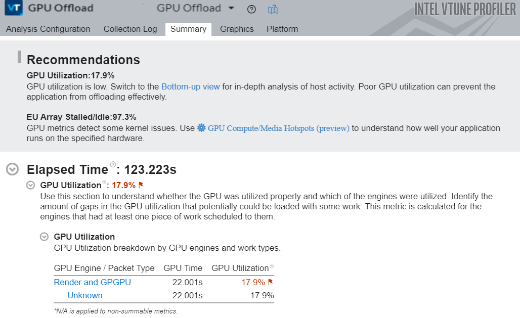
Once the analysis is complete, the Summary window informs us about measurements of GPU Utilization and EU Stalls. Following the recommendations here, let us first examine host activity that could be responsible for low GPU utilization. We switch to the Graphics tab to open the Bottom-up view.
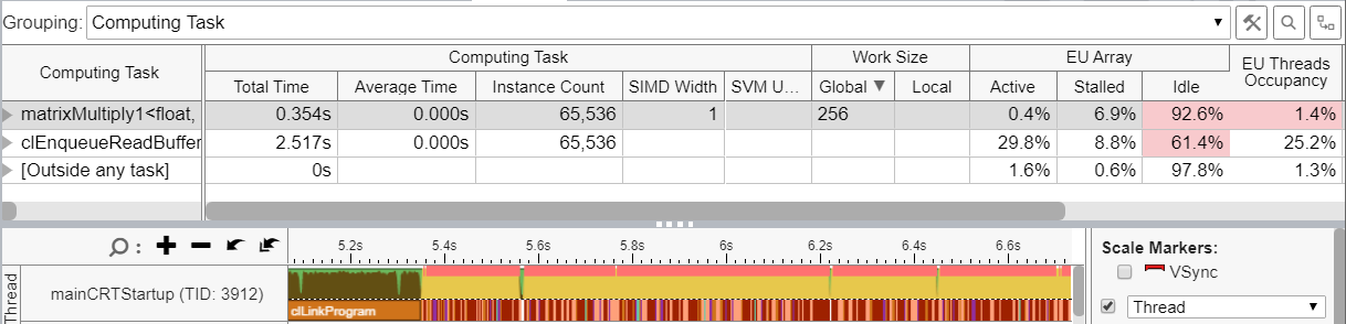
Look at the matrixMultiply1 kernel results in the figure above.
In order to get the work completed in a reasonable amount of time, this version of the kernel uses 256X256 dimension matrices. The Instance Count column tells us that the kernel was invoked 65,536 times. Each instance was so small that the average time of the kernel was rounding off to zero seconds. The spectrum pattern in the timeline also indicates a rapid kernel invocation rate. In this case, most of the time is spent on creating small kernels. The Idle column in the EU Array section informs us that the EUs were idle for 92.6% of the time. Invoking too many short kernels is a key indicator of work inefficiency.
The Work Size section reveals that there was inefficiency in work distribution. Let us now offload the outer loop.
This action should give better performance by reducing the number of compute kernel instances to one (matrixMultiply2). The figure below shows a GPU Hotspots analysis for this improved version of the kernel. This version is also called a Naïve implementation.

In this case, the size of the matrices was increased to 2048 X 2048 and the wall-clock performance was still more than 10x faster. The EU Threads Occupancy metric is high. This indicates that there is enough work available for the execution units.
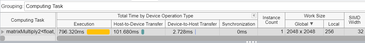
When we look at the timeline in the figure above, we observe a single computing task that took nearly 800 ms, versus data transfer that only took 100 ms. This ratio between executing data and transferring data is more desirable. Further improvements to the algorithm can result in greater improvements to this ratio.
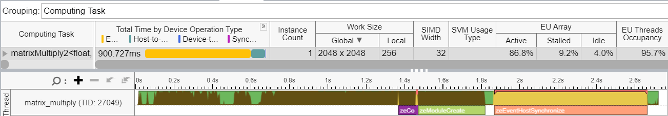
Notice that the compiler generated the full length of SIMD instructions (SIMD Width=32). This arranged data access that resulted in the EUs being active for 86.8% of the time, as opposed to near zero in the previous run. This exercise demonstrates the importance of providing enough work within each invocation of a kernel.
The naive implementation of the matrix multiplication example is much faster than the initial version. But we can still expect improvements in performance.
VTune Profiler reported a high value for the EU Threads Occupancy metric (95.7%), which meant that the work was distributed properly among EUs. But the execution engine is still underutilized with the matrixMultiply2 kernel. We deduce this from the EU Array Stalled metric, which is only 9.2%.
To investigate limiting factors for a kernel, let us run the GPU Compute/Media Hotspots analysis. This way, we can see detailed information about kernel execution in a GPU.
Our first step is to identify if the kernel is computed bound or memory bound.
The GPU Hotspots analysis has several predefined profiles or presets. You can use these presets to collect different metrics related to memory access and computing efficiency. To understand kernel execution better, we use the Full Compute preset. From the information in this preset, we see that EU FPUs were only active 63.5% of the time by executing the kernel matrixMultiply2.

Therefore, the kernel was memory bound, not compute bound.
Our next step is to examine the Memory Hierarchy Diagram. This diagram provides data transfer information between EUs and memory units. The information can help us define optimization steps in the code of the kernel.
When we select the Overview preset, the Memory Hierarchy Diagram displays values for the bandwidth of the links between memory units (like GPU L3 Cache, GTI Interface, LLC and DRAM) and EUs, as well as total data transferred between them.
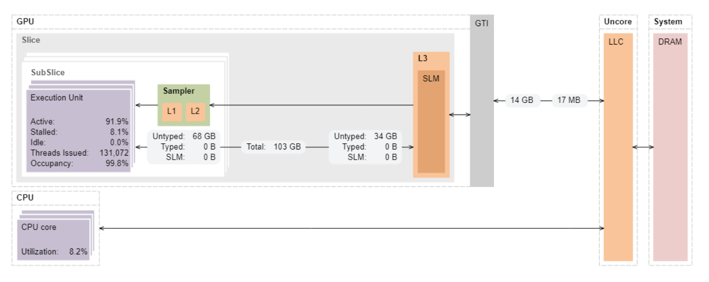
Notice the overall amount of data transferred to EUs (~68 GB) and data brought from LLC/DRAM through the GTI interface (14 GB).
When you compare these data sizes to the size of each matrix data array (2048x2048x4=16MB), the transferred amount is enormously high. This condition makes execution ineffective due to access to global memory. We should address this issue with more efficient data access (a consequent data or unit stride access in array) and minimal access to the global memory.
Fetching data from global memory is a common performance limiting factor for GPUs. This problem is worsened in the case of discrete GPUs. Here, the PCIe bus introduces more bandwidth and latency limitations. A common but sub-optimal approach is to increase data locality and reuse. This is done by blocking matrix areas and completing multiply-add operations within the smaller blocks that fit into a cache memory that resides closer to execution units. You can implement this optimization by one of two ways:
- Allow the hardware to recognize frequently accessed data and preserve it in a cache automatically.
- Exercise more manual control over access to data blocks by placing the most used data in the Shared Local Memory.
Use care when implementing the latter as it can result in these conditions:
- Poor management of threads, as SLM access is limited to threads from its slice only.
- Slow data access in case the ratio of data reads/write is below a certain threshold.
One approach to use SLM with the matrix multiplication algorithm is to split the global work set of matrices into blocks or tiles and perform dot product operations in the tiles separately. This action should decrease the number of global memory accesses as the entire tile should fit into the SLM area. Although this approach does not enable optimal access to data arrays, the access is much faster due to achieved data locality.
In the code snippet below, the pseudo code demonstrates the idea of data accesses to tiles in the local index space.
i, j // global idx
    for (size_t tidx = 0; tidx < TILE_COUNT; tidx++)
         ti, tj // local idx
         ai, aj, bi, bj // global to local idx
         ta[ti, tj] = a[ai, aj]
         tb[ti, tj] = b[ai, aj]

         for (size_t tk = 0; tk < TILE_SIZE; tk++)
                c[i][j] += ta[ti][tk] * tb[tk][tj];
     }
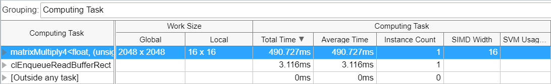
The implementation of the tiled multiplication significantly redistributes the data flow. An analysis of the matrixMultiply4 kernel (see Memory Hierarchy diagram below) reveals some observations:
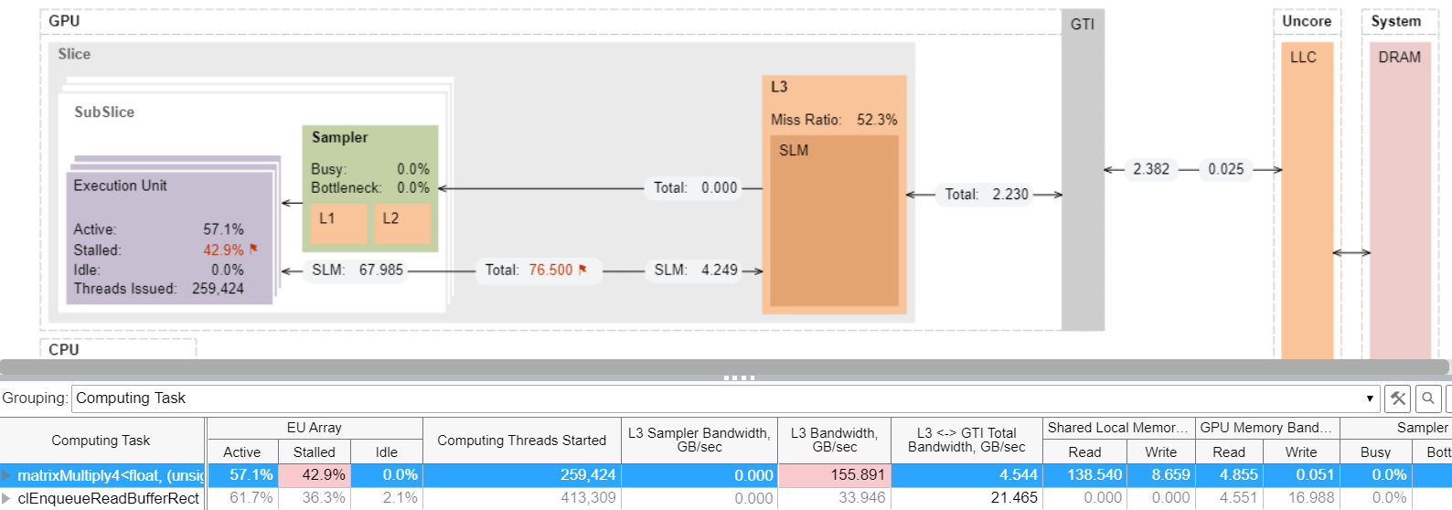
- The data volume coming from LLC via GTI interface is just ~2 GBs, most of which came from L3/SLM.
- The L3 Bandwidth metric (highlighted in the table above) reached 155GB/s, which is more than 70% of the maximum L3 bandwidth.
- 42% of EUs were still stalled.
From these observations, we can conclude that the algorithm execution is still memory bound, albeit with much faster cache memory. In total, the kernel now executes almost 5x faster than the naïve implementation we started with.
Next, let us look at the total time for computing tasks, as shown in the table below.
There are a few ways in which we can enable a faster implementation.
- Organize high level data access in a more optimal way.
Using sub-groups for data distribution, we can leverage sub-slices of the GPU that access their own local memory.
- Use a low-level optimization for specific GPU architecture and use optimized libraries like Intel® oneAPI Math Kernel Library (oneMKL).
These steps can help us achieve near maximum performance with the GPU. However, any GPU has its theoretical limit for performance that can be calculated using some known characteristics.
For example, let us calculate the theoretical minimum time for algorithm execution in the Gen9 GPU. From the Gen9 GT2 GPU architecture parameters, we know that this GPU contains 24 EUs. Each EU has two FPUs (SIMD-4). Each FPU can perform two operations (MUL+ADD). With a max core frequency of 1.2 GHz, the maximum FP performance is:
24 * 2 * 4 * 2 = 384 Flop/cycle (32b float)
384 * 1.2 = 460.8 GFLOPS
The number of FP operations of the naïve matrix multiplication implementation is 2*N3, which is approximately 17.2 GOPS when N=2048.
Theoretically, if we were not limited by data access inefficiency and bandwidth constraints, the algorithm could be calculated in 17.2 / 460.8 = 0.037 sec or 37 ms. The VTune results revealed that the best time executed by the kernel was 490 ms, which is over 10x slower than the theoretical calculation time. We can therefore conclude that there is still room for performance improvement.
A highly parallel application, like the matrix multiplication sample, leverages the increased efficiency from the use of GPU resources. However, using additional compute resources should also increase performance, provided the scaling is not limited by memory bottlenecks.
In the Gen9 series of GPUs, there are GT3 and GT4 options, which contain 48 EUs and 72 EUs respectively. However, embedded GPUs have a fundamental limitation in area. This prevents us from adding more EUs for greater potential scaling, and bigger cache blocks for faster data access. Discrete GPUs are less limited by area or power constraints. If a system allows integration with a single, external GPU or with multiple GPUs, we could scale up accelerator performance.
However, remember that between the main CPU, its memory, and the GPU, there will be a communication interface (like a PCIe bus). This may have its own constrains on bandwidth, latency, and data coherency.
Let us look at an Intel® Iris® Xe MAX GPU, previously known as a PCIe discrete graphics card with the code name DG1.
An analysis of the same tiled kernel implementation gives us these results:
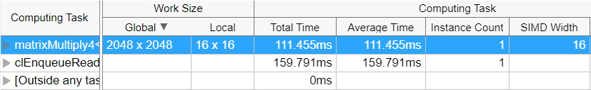
The kernel execution is roughly 4x faster.
This is expected, as the Intel® Iris® Xe MAX GPU has 96 EUs against the 24 EUs in the observed Gen9 GPU. However, we can notice in the table below that the EUs are still stalled 51% of the time during execution. This is quite likely due to the wait for data from memory (which is well known for general matrix algorithms). The question is, which one?

If we switch the mode in the results grid to show the percentage of maximum bandwidth, we observe that the L3 and GPU memory bandwidth was far from the maximum, so they are not bottlenecks. Let us look at the Memory Hierarchy Diagram to get a better picture of data transfers.
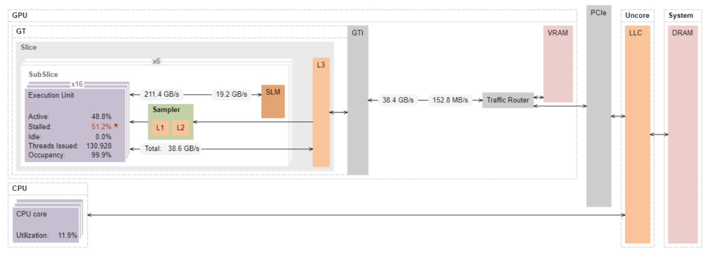
Beyond the GTI interface, data comes from the VRAM or main DRAM. As we prepare matrix data on the CPU side, we know that data for matrix a and matrix b is transferred via PCIe to the GTI. The measured GTI bandwidth is a rough indication of the data rate required for PCIe interface. The measured data read rate is 38 GB/s at the GTI interface, while PCIe 3.0x16 has a theoretical maximum of only16GB/s one way. A reasonable conclusion is that we are limited to the PCIe bandwidth. To measure the data traffic on PCIe with VTune Profiler, we need a server platform, which has PCIe performance counters.
On a server-based setup, the bandwidth on the PCIe is much lower than bus limitations. So, we can conclude that:
- All data is being fetched from VRAM and the EU stalls. This may be defined by the latency of traveling data from video memory to EUs.
- Since the data traffic between EUs and L3 is the same as between GTI and the external traffic router, you can achieve additional performance optimizations using a better reuse of the L3 cache. For example, you can introduce second level of matrix tiling with blocks size that would fit to the L3 cache of each GPU slice.
Conclusion
Generally, in heterogeneous applications, once a certain workload is offloaded onto an accelerator, it is essential to provide enough computing tasks for massively parallel accelerator machines like a GPU.
- Improve the efficiency of the GPU by estimating the data transfer and task scheduling overhead for offloaded tasks.
- Use the GPU Utilization and GPU Occupancy metrics in the GPU Offload analysis of VTune Profiler to estimate the inefficiency of using a GPU.
- The performance of a computing task execution may be limited by several microarchitectural factors, like the lack of Execution Units or presence of bottlenecks in memory subsystems or interfaces. Run the GPU Compute/Media Hotspots analysis to identify these limitations. Highlight the bottlenecks on the GPU Memory Hierarchy Diagram along with detailed microarchitecture metrics for every computing task. For more complicated kernels, use the latency analysis to identify the most critical code inside a kernel.