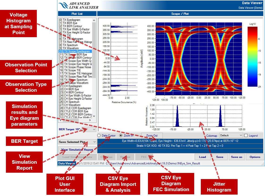
2.2. Intel® Advanced Link Analyzer Data Viewer Module
The Intel® Advanced Link Analyzer Data Viewer displays simulation and analysis results. The Data Viewer can be started in the following ways:
- Automatically start after the completion of a simulation.
- Click Data View in Intel® Advanced Link Analyzer’s main GUI.
- Double-click adv_link_analyzer_data_viewer.exe.
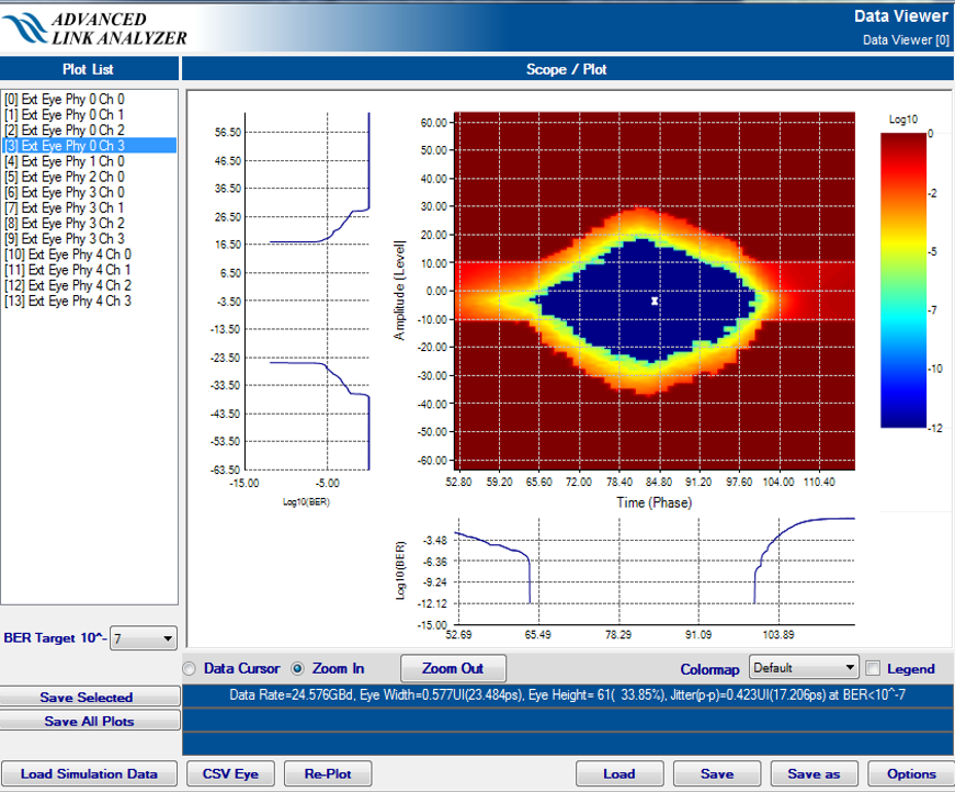
Intel® Advanced Link Analyzer uses the Data Viewer to show various types of simulation and analysis results. It can show multiple plots. Use the list box in the left panel to select the plots.
The following GUI capabilities are provided in the Data Viewer:
- Zoom control
- In an eye diagram plot—Click Zoom In or click and drag a rectangle box to show the details of a plot. Click Zoom Out to restore the plot scale.
- Others—Right-click to bring up a menu with Zoom Out, Select, Zoom, Pan, and waveform commands.
- Data Cursor—Select Data Cursor to show the data cursor boxes. You can select and drag a data cursor box with the data values shown in the box. The data values are colored according to the data lines.
Note: The Data Cursor button may not be present in certain types of plots such as waveform plots. If you move the cursor over a data point, a pop-up window shows the data value.
- Legends—Plot legends are shown when plots are generated. Use the Page-Up, Page-Down, Home, and End keys on the keyboard to move the legend box. Turn the Legends on or off to show or hide the legend box.
Within the Data Viewer, you can modify the link’s BER target using the BER Target menu. The Intel® Advanced Link Analyzer Data Viewer recalculates the jitter and the eye-opening height and width dynamically, because the Intel® Advanced Link Analyzer Simulation Engine has pre-calculated the results at different BER targets in the simulation range.
Use the Colormap menu to change the color map of eye diagrams within the Data Viewer. Intel® Advanced Link Analyzer provides eight different color maps that you can choose from, depending on your analysis purpose and visual preferences. The color maps can be divided into two groups:
- Logarithmic Color Scale—Default, Blue, Heat, and Bone
- Linear Color Scale—Default Linear, Blue Linear, Heat Linear, and Bone Linear
The logarithmic color scale provides good visual performance in displaying low probability data points such as the low BER portion of an eye diagram. The linear color scale is more suitable for showing minor differences in close-range data values. The Blue/Blue Default Linear is good for showing deterministic simulation results when no jitter or noise is present. Intel® Advanced Link Analyzer automatically chooses the most suitable color map based on the type or configuration of a simulation. The default color map is either Default or Blue.
- When Save Selected Plot is selected, the image of the currently selected plot is generated and saved. An image file of the currently selected plot is saved in the format specified in the Image Output (in the Options window).
- When Save All Plots is selected, the images of all plots are generated and saved to the folder you specify. Image files of all plots are saved in the format specified in the Image Output (in the Options window).
- When Save Waveform is selected, you specify the file name and location to save the waveform data. Note that you must first select a waveform plot to save the waveform data.
- When Save Simulation Report is selected, a simulation report in XML format is generated and saved to the folder you specify. To share the simulation report, you must include the generated XML file (for example, Your_Sim.xml) as well as the folder (for example, Your_Sim_SimResults) for the simulation report to display correctly.
- When View Simulation Report is selected, a media-rich simulation report in XML format is generated and displayed in an XML viewer. You can use any XML viewer to view the simulation report.
The Intel® Advanced Link Analyzer Data Viewer Module shows the following types of simulation results:
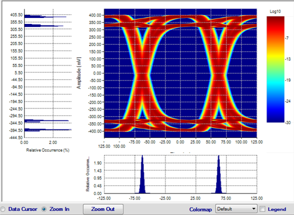
Probability Density Function (PDF) Eye Diagram
This scope shows the PDF eye diagram (with probability color map), horizontal histogram at slicer voltage level (fixed at 0 V in the Intel® Advanced Link Analyzer), vertical histogram at Ideal Clock or CDR sampling phase, and eye diagram opening width and height information. Device settings such as transmitter pre-emphasis/FIR setting and receiver equalization settings are shown in the text display area below the plots.
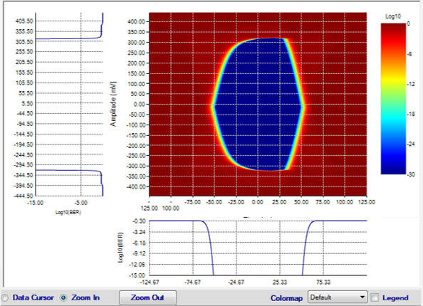
Cumulative Distribution Function (CDF) Eye Diagram
This scope shows the CDF eye diagram (with probability color map), horizontal BER bathtub curve (fixed at 0 V in Intel® Advanced Link Analyzer), vertical BER bathtub curve (at ideal clock or CDR sampling phase), and eye diagram opening width and height. The eye diagram compliance mask is plotted when it is enabled and applicable.
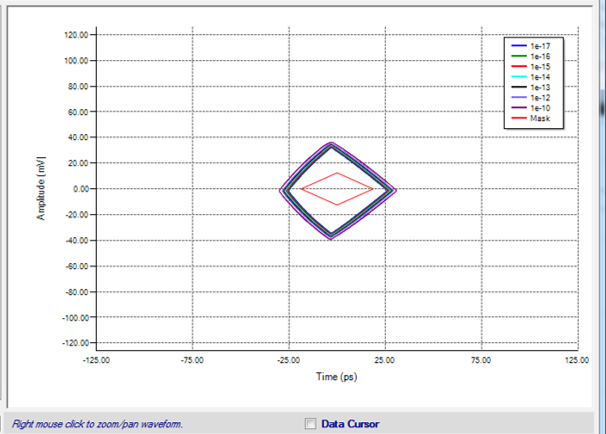
BER Contour
The Data Viewer shows the BER contour and eye diagram opening width and height. The eye diagram compliance mask is plotted when it is enabled and applicable.
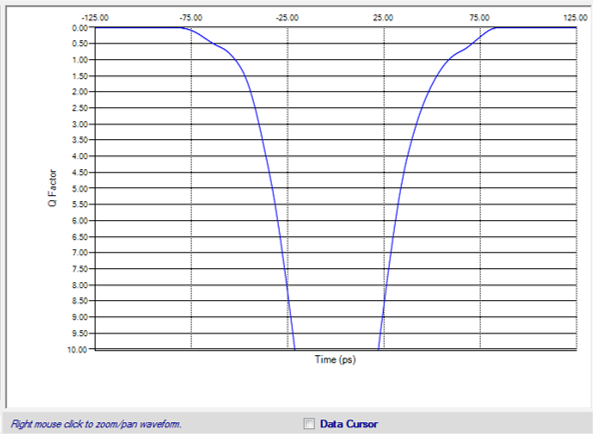
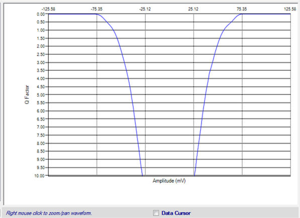
Q-Factor Curve
A different view of the BER bathtub curve using Q-factor.
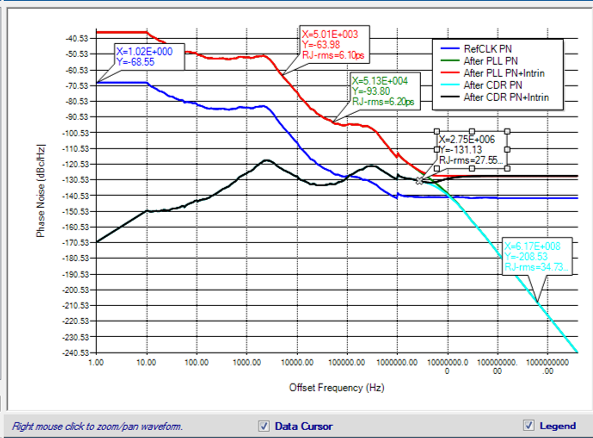
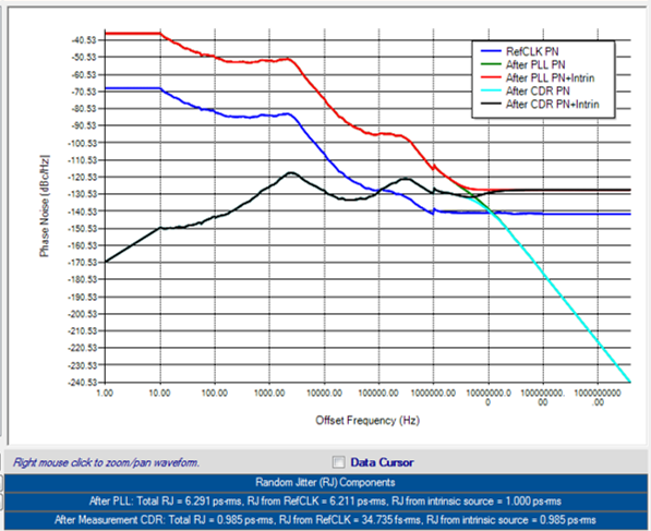
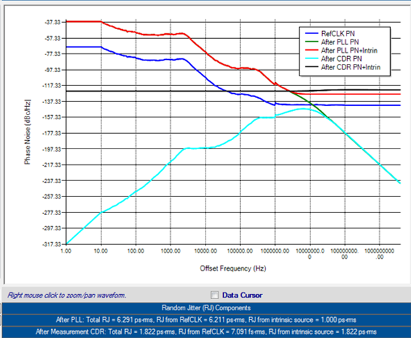
Transmitter Reference Clock Phase Noise Analysis and Plots
Intel® Advanced Link Analyzer plots the phase noise power spectrum through the link. The transmitter reference clock’s phase noise travels through the transmitter PLL, emulated scope, channel, and the RX CDR. In this process, phase noise is shaped by the TX PLL, scope (pass through only), and RX CDR. At the same time, the transmitter and receiver also generate their own intrinsic jitter which is mixed with the jitter caused by the shaped phase noise. The Intel® Advanced Link Analyzer simulation engine processes and records the phase noise characteristics transition and the amount of random jitter the device contributed internally.
TX pre-emphasis, de-emphasis, or FIR coefficients are displayed with the transmitter output.
The CTLE setting is displayed for the test point after CTLE.
DFE coefficients are displayed for the test point after DFE.
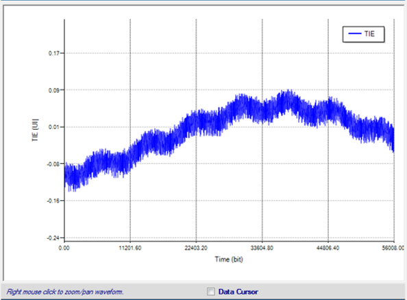
Time Interval Error (TIE) Plots
TIE plots capture the time differences between the waveform transition time (across data sensing threshold) and ideal/reference waveform transition time. If Jitter Analysis is enabled and the simulation mode is Hybrid, jitter analysis results are displayed under the TIE plot.
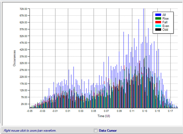
Time Interval Error (TIE) Histogram Plots
This plot shows the histogram of TIE records. Five histograms are displayed:
- All transitions
- Rising edge transitions
- Falling edge transitions
- Even-bit edge transitions
- Odd-bit edge transitions
If Jitter Analysis is enabled and the simulation mode is Hybrid, jitter analysis results are displayed under the TIE plot.
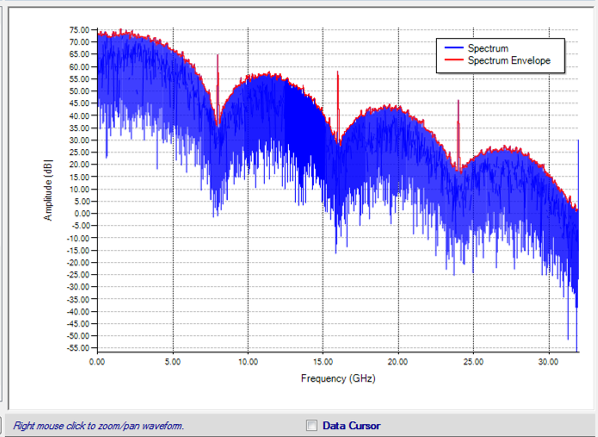
Waveform Spectrum Plots
The frequency spectrum of the waveform is plotted.
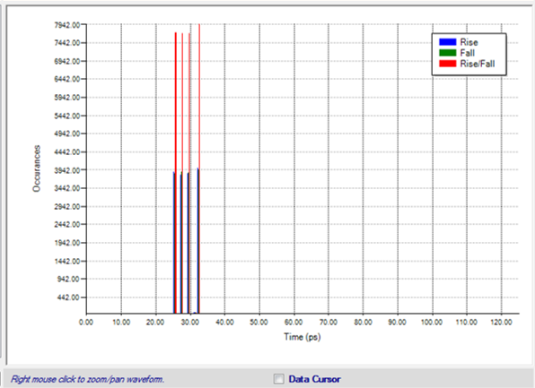
Rise/Fall Time Histogram Plots
Intel® Advanced Link Analyzer calculates the rise/fall time across the bit time boundary.
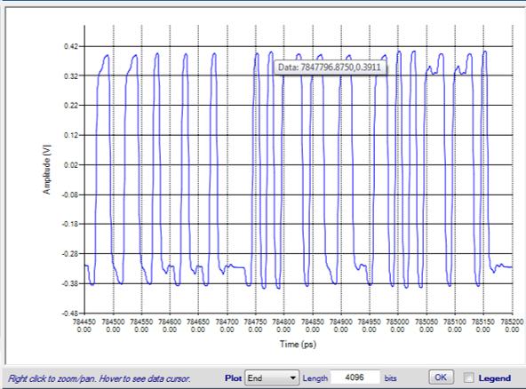
Waveform
For Hybrid mode or Full Waveform mode simulations, a waveform of each test point is plotted. The Data Viewer, by default, displays the final 4096 bits of the waveform. Use the following settings to specify the location of the waveform:
- Plot—The Plot menu specifies the reference location of the simulated waveform. It has the following choices:
- Beginning—plots the waveform from the beginning of the simulation.
- End—displays the last part of simulated waveform.
- Custom—you specify the starting and ending bit locations.
- Length—If the Plot selection is Beginning or End, the length of waveform (in bits) to be plotted is specified.
- From/to—If the Plot selection is Custom, these two entries specify the start and end points of waveform (in bits) to be plotted.
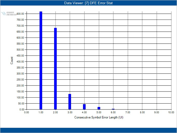
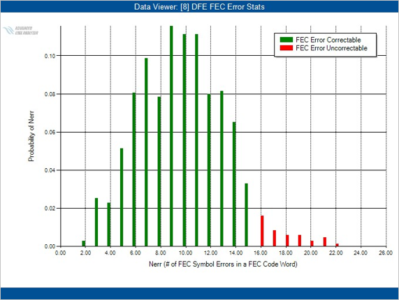
Symbol/FEC Error Analysis
For Hybrid mode or Full Waveform mode simulations with FEC enabled and symbol/FEC error analysis enabled, the simulation engine computes the symbol error statistics and FEC code word error statistics. In the symbol error statistics plot, the X-axis is the consecutive symbol error length, (burst symbol error length) and the Y-axis is the occurrence count. In the FEC code word error statistics plot, the X-axis is the number of FEC symbol errors in a FEC code word, denoted as Nerr, and the Y-axis is the probability of Nerr. The FEC code word error statistics plot is color-coded where green bars represent correctable FEC code words and red bars represent uncorrectable FEC code words. Only the uncorrectable FEC code words result in bit errors after the receiver’s FEC decoder. The correctable/uncorrectable threshold is determined based on the FEC configuration of the simulated serial link.
- If the link does not induce symbol errors, the symbol/FEC error analysis plot is not shown.
- FEC error analysis supports serial links with the Reed-Solomon error correction scheme.
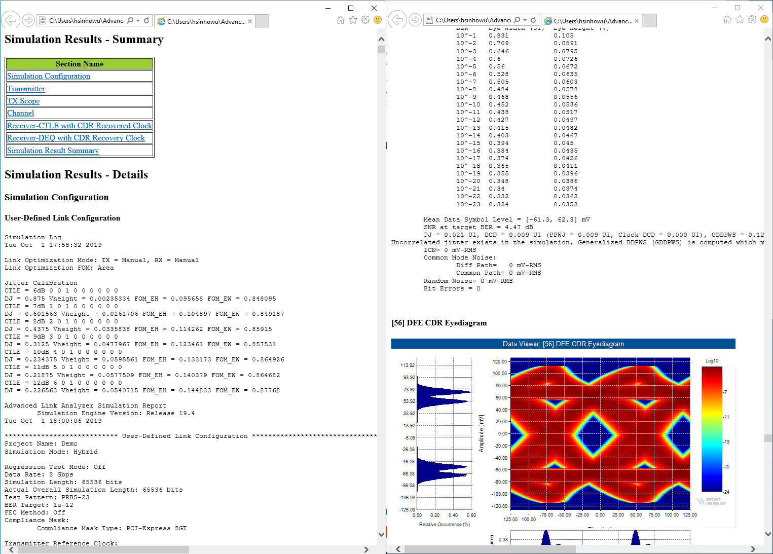
Simulation Report
A simulation report is shown in the last page of the output windows. The simulation report is organized as follows:
- Simulation Log—If link optimization is performed, the link optimization FOM (figure of merit) transition is reported here.
- User-Defined Link Configuration—Link configuration is listed in this section which includes:
- Transmitter Reference clock configuration
- Transmitter configuration
- Receiver configuration
- Channel configuration
- Simulation Record—Report the simulation results at each test points
- Simulation Result Summary
- TX-FIR/Pre-emphasis, RX CTLE, and DFE Settings
- Eye Diagram Widths, Heights, and Margins to the eye diagram mask
---------------------------------------------------------------
Simulation Log
<current date>
Link Optimization Mode: TX = Manual, RX = Manual
Link Optimization FOM: Area

               Intel® Advanced Link Analyzer Simulation Report
 Simulation Engine Version: <current version>
**************************** User-Defined Link Configuration ********************************
Project Name: Demo
Simulation Mode: Hybrid
Data Rate: 8 Gbps
Simulation Length: 65536 bits
Test Pattern: PRBS-23
BER Target: 1e-012
FEC Method: Off
Compliance Mask:
 Compliance Mask Type: PCI-Express 8GT
Transmitter Reference Clock:
 Frequency: 100 MHz
 Configuration Method: Option 2
  Phase Noise Profile [Freq (Hz), Amplitude (dBc)]:
   [10, -68.5508]
   [10.2723, -68.7007]
   [10.552, -69.0572]
   [10.8393, -69.5463]
   [11.1344, -69.8799]
   [11.4376, -70.1791]
...
   [8.98118e+007, -141.908]
   [9.22571e+007, -141.914]
   [9.47691e+007, -141.916]
   [9.73494e+007, -141.9]
   [1e+008, -142.145]
  Phase Noise Fmin: 1 Hz
  Phase Noise Fmax: 1e+008 Hz
  Spur Profile [Freq (Hz), Amplitude (dBc)]:
   [100000, -80]
   [1e+006, -90]
   [1e+007, -96]
  Periodic Jitter:
   Method: Triangle
   Frequency: 0 Hz
   Amplitude: 0 ps
  Hershey Key: 0.05
  Sharkfin Key: 0.5
Transmitter: Stratix V GX
 Package: Stratix V GX
 Supply Voltage: Default
 Vcm: Default
 PLL Type: Enable
  PLL Bandwidth: SVGX_TXPLL_Low
  Divider Setting: L = 1, M = 40, N = 1
 VOD: 0.8 V
 TX EQ/FIR Mode: Manual
 Initial TX FIR Coefficients = [-4, Main Tap, 2, 0]
 PVT Condition:
  PVT: Typical
 Jitter & Noise Configuration:
  Jitter/Noise Input Method: Jitter/Noise Component Method
  ISI = 0 ps
  DCD = 1.5 ps
  BUJ = 4 ps
  RJ = 1 ps-rms
  SJ = 0 ps at 0 MHz
  DN = 0 mV
  BUN = 0 mV
  RN = 0 mV-rms
Receiver: PCI-Express 8GT
 Package: PCI-Express 8GT
 Supply Voltage: Default
 CTLE Mode: 10dB
 CDR Type: Alexander
  CDR Bandwidth: Generic_CDR_Medium_BW
 DFE Enable: Enable
 DFE Mode: Auto
 PVT Condition:
  PVT: Typical
 Jitter & Noise Configuration:
  Jitter/Noise Input Method: Jitter/Noise Component Method
  DJ = 7 ps
  BUJ = 0 ps
  RJ = 1.55 ps-rms
  DN = 0 mV
  BUN = 0 mV
  RN = 0 mV-rms
Channel Configuration:
 [1] File Name: Demo.s12p
  Channel Type: Loss
  Port Configuration: 2
  Lane Number: 2
  Port Number: 12
  Aggressor ID: 1
  Aggressor Relative Amplitude: 1
  Aggressor Delay: 0
  Aggressor Frequency Offset: 0 ppm
  Aggressor Signal Source Type: Inline
  Causality Enforcement: No
  Passivity Enforcement: No
 [2] File Name: Demo.s12p
  Channel Type: FEXT
  Port Configuration: 2
  Lane Number: 2
  Port Number: 12
  Aggressor ID: 1
  Aggressor Relative Amplitude: 1
  Aggressor Delay: 0
  Aggressor Frequency Offset: 0 ppm
  Aggressor Signal Source Type: Inline
  Causality Enforcement: No
  Passivity Enforcement: No
 [3] File Name: Demo.s12p
  Channel Type: FEXT
  Port Configuration: 2
  Lane Number: 2
  Port Number: 12
  Aggressor ID: 2
  Aggressor Relative Amplitude: 1
  Aggressor Delay: 0
  Aggressor Frequency Offset: 300 ppm
  Aggressor Signal Source Type: Inline
  Causality Enforcement: No
  Passivity Enforcement: No
****************************************************************************************************************
******************************************* Simulation Record **************************************************
Transmitter Reference Clock Random Jitter = 6.37602 ps-RMS (up to Reference Clock Frequency)
TX with Ideal Clock
 Stratix V GX VOD: 40 TX EQ: Pre-Tap 1 = -4 Post-Tap 1 = 2 Post-Tap 2 = 0
 Eye Width=0.17UI(21.240ps), Eye Height=  363.49mV, Jitter(p-p)=0.83UI (103.760ps) at BER<10^-12
  BER Eye Width (UI) Eye Height (V)
  10^-3 0.622  0.632
  10^-4 0.545  0.62
  10^-5 0.48  0.607
  10^-6 0.424  0.593
  10^-7 0.373  0.574
  10^-8 0.326  0.552
  10^-9 0.284  0.524
  10^-10 0.243  0.486
  10^-11 0.205  0.431
  10^-12 0.17  0.363
  10^-13 0.136  0.288
  10^-14 0.103  0.21
  10^-15 0.0713  0.132
  10^-16 0.041  0.0529
  10^-17 0.00977  0
  10^-18 0  0
  10^-19 0  0
  10^-20 0  0
  10^-21 0  0
 Random Jitter= 6.29 ps-RMS
 Random Noise= 0 mV-RMS
TX Scope with Recovered Clock
 Stratix V GX VOD: 40 TX EQ: Pre-Tap 1 = -4 Post-Tap 1 = 2 Post-Tap 2 = 0
 Eye Width=0.83UI(104.126ps), Eye Height=  636.61mV, Jitter(p-p)=0.17UI (20.874ps) at BER<10^-12
  BER Eye Width (UI) Eye Height (V)
  10^-3 0.915  0.642
  10^-4 0.899  0.64
  10^-5 0.888  0.639
  10^-6 0.877  0.638
  10^-7 0.868  0.638
  10^-8 0.86  0.638
  10^-9 0.853  0.638
  10^-10 0.845  0.638
  10^-11 0.839  0.637
  10^-12 0.833  0.637
  10^-13 0.827  0.637
  10^-14 0.821  0.637
  10^-15 0.816  0.637
  10^-16 0.812  0.637
  10^-17 0.807  0.637
  10^-18 0.802  0.637
  10^-19 0.798  0.636
  10^-20 0.794  0.636
  10^-21 0.788  0.636
 Random Jitter= 0.985 ps-RMS
 Random Noise= 0 mV-RMS
CH
 Eye Width=0.00UI( 0.000ps), Eye Height=    0.00mV, Jitter(p-p)=1.00UI (125.000ps) at BER<10^-12
  BER Eye Width (UI) Eye Height (V)
  10^-3 0  0
  10^-4 0  0
  10^-5 0  0
  10^-6 0  0
  10^-7 0  0
  10^-8 0  0
  10^-9 0  0
  10^-10 0  0
  10^-11 0  0
  10^-12 0  0
  10^-13 0  0
  10^-14 0  0
  10^-15 0  0
  10^-16 0  0
  10^-17 0  0
  10^-18 0  0
  10^-19 0  0
  10^-20 0  0
  10^-21 0  0
 Random Jitter= 6.29 ps-RMS
 Random Noise= 0 mV-RMS
CTLE CDR with Recovered Clock
 CTLE Setting: 10dB
 Eye Width=0.44UI(55.298ps), Eye Height=   41.99mV, Jitter(p-p)=0.56UI (69.702ps) at BER<10^-12
  BER Eye Width (UI) Eye Height (V)
  10^-3 0.689  0.0562
  10^-4 0.637  0.0512
  10^-5 0.586  0.0485
  10^-6 0.547  0.047
  10^-7 0.521  0.0459
  10^-8 0.502  0.045
  10^-9 0.484  0.0444
  10^-10 0.47  0.0437
  10^-11 0.455  0.0426
  10^-12 0.442  0.042
  10^-13 0.431  0.0411
  10^-14 0.42  0.0405
  10^-15 0.409  0.0398
  10^-16 0.399  0.0389
  10^-17 0.391  0.0385
  10^-18 0.381  0.0376
  10^-19 0.372  0.037
  10^-20 0.363  0.0363
  10^-21 0.355  0.0356
 Random Jitter= 1.84 ps-RMS
 Random Noise= 0 mV-RMS
 DFE CDR with Recovered Clock
 DFE Coefficients = [   -19.73,] mV
 Eye Width=0.41UI(51.392ps), Eye Height=   60.06mV, Jitter(p-p)=0.59UI (73.608ps) at BER<10^-12
  BER Eye Width (UI) Eye Height (V)
  10^-3 0.616  0.0881
  10^-4 0.567  0.0812
  10^-5 0.532  0.0763
  10^-6 0.507  0.0726
  10^-7 0.485  0.0697
  10^-8 0.467  0.0672
  10^-9 0.451  0.065
  10^-10 0.438  0.063
  10^-11 0.424  0.061
  10^-12 0.411  0.0601
  10^-13 0.4  0.0581
  10^-14 0.39  0.0571
  10^-15 0.379  0.0554
  10^-16 0.369  0.0542
  10^-17 0.36  0.0529
  10^-18 0.351  0.0517
  10^-19 0.343  0.0505
  10^-20 0.333  0.049
  10^-21 0.325  0.0485
 Random Jitter= 1.84 ps-RMS
 Random Noise= 0 mV-RMS
*******************************************************************************************************
Simulation Result Summary
**************************** TX-FIR/Pre-emphasis, RX CTLE and DFE Settings ****************************
Pre-emphasis : Pre-tap1  main-tap  Post-tap1  Post-tap2
 Levels : -4.000  0.000  2.000  0.000
 Coeff : -0.087  0.962  -0.041  0.000
RX Setting : CTLE Setting: 10dB
DFE  : tap1
****************************************************************************************************************
******************************** Eyediagram Width and Eyediagram Height ****************************************
    Eye Width Eye Height Eye Opening
    [UI]  [V]  Area [UI*V]
TX Output (Scope)  : 0.833  0.637  0.530
TX Output  : 0.170  0.363  0.062
Channel Output  : 0.000  0.000  0.000
CTLE Output (Retimed) : 0.442  0.042  0.019
DFE Output (Retimed) : 0.411  0.060  0.025
 Eye Mask Margin : 0.111  0.035
****************************************************************************************************************
Simulation Time: 0:04:27.70
Simulation Time: 0:04:34.55

--------------------------------------------------------------------
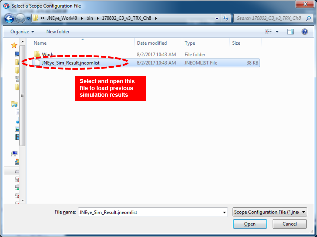
Use the Data Viewer to see previous Intel® Advanced Link Analyzer simulation results by clicking Load. A file browser opens and helps you find the master Intel® Advanced Link Analyzer output data file (JNEye_Sim_Result.jneomlist) for individual simulations. Intel® Advanced Link Analyzer simulation output data is usually located in a file directory that has the same name as the saved project name. For example, if the saved Intel® Advanced Link Analyzer configuration file is Demo1.jne, the previous simulation results are stored a directory named “Demo1”. Navigate to the directory, select the JNEye_Sim_Result.jneomlist file, and open it to load the simulation data.
CSV Eye Diagram Import and Analysis
Eye diagram data generated from other simulation tools or measurement instruments can be imported and analyzed in Intel® Advanced Link Analyzer’s Data Viewer. After valid eye diagram data is imported, the Data Viewer performs BER bathtub and eye height/width analysis. The Data Viewer is equipped with options to repair or enforce the integrity of the imported CSV data.
Two CSV eye diagram data formats are supported:
CSV Eye Diagram Data Format 1: Format 1 includes a predefined header section which is followed by a 2-dimension data array.
Required headers for the CSV eye diagram data:
- Datarate: Datarate of the measured eye diagram
- Optimum phase: Phase where the eye height opening is optimal
- Eye measured at vertical step: Amplitude where the eye width is measured
- Header text: Name of the measurement data
- Dimension X-axis: X-axis dimension of the measured data
- Dimension Y-axis: Y-axis dimension of the measured data
- START: Starting point of eye diagram data
Example of Format 1 eye diagram data:
======================================================================
>>>>,Datarate Ch  0 phy 0                   : ,24576,Mbps
>>>>,Horizontal Eye Opening Ch  0 phy 0     : ,35,phases
>>>>,Horizontal Eye Opening Ch  0 phy 0     : ,0.55,UI
>>>>,Optimum Phase Ch  0  phy 0             : ,85
>>>>,Eye measured at vertical step          : , 2
>>>>,Vertical Eye Opening Ch  0 phy 0       : ,45,steps
>>>>,Area Eye Opening Ch 0 phy 0            : ,1139
>>>>,Header Text,Phy 0 Ch  0
>>>>,Dimension X-axis,64
>>>>,Dimension Y-axis,127
>>>>,=============================================================================================
>>>>,
>>>>,START,
>>>>,Phase   ,53,54,55,56,57,58,59,60,61,62,63,64,65,66,67,68,69,70,71,72,73,74,75,76,77,78,79,80,81,82,83,84,85,86,87,88,89,90,91,92,93,94,95,96,97,98,99,100,101,102,103,104,105,106,107,108,109,110,111,112,113,114,115,116,
>>>>,63     ,1.000000e+00,1.000000e+00,1.000000e+00,1.000000e+00,1.000000e+00,1.000000e+00,1.000000e+00,1.000000e+00,1.000000e+00,1.000000e+00,1.000000e+00,1.000000e+00,1.000000e+00,1.000000e+00,1.000000e+00,1.000000e+00,1.000000e+00,1.000000e+00,1.000000e+00,1.000000e+00,1.000000e+00,1.000000e+00,1.000000e+00,1.000000e+00,1.000000e+00,1.000000e+00,1.000000e+00,1.000000e+00,1.000000e+00,1.000000e+00,1.000000e+00,1.000000e+00,1.000000e+00,1.000000e+00,1.000000e+00,1.000000e+00,1.000000e+00,1.000000e+00,1.000000e+00,1.000000e+00,1.000000e+00,1.000000e+00,1.000000e+00,1.000000e+00,1.000000e+00,1.000000e+00,1.000000e+00,1.000000e+00,1.000000e+00,1.000000e+00,1.000000e+00,1.000000e+00,1.000000e+00,1.000000e+00,1.000000e+00,1.000000e+00,1.000000e+00,1.000000e+00,1.000000e+00,1.000000e+00,1.000000e+00,1.000000e+00,1.000000e+00,1.000000e+00,
>>>>,62     ,1.000000e+00,1.000000e+00,1.000000e+00,1.000000e+00,1.000000e+00,1.000000e+00,1.000000e+00,1.000000e+00,1.000000e+00,1.000000e+00,1.000000e+00,1.000000e+00,1.000000e+00,1.000000e+00,1.000000e+00,1.000000e+00,1
…
…
>>>>,-62    ,1.000000e+00,1.000000e+00,1.000000e+00,1.000000e+00,1.000000e+00,1.000000e+00,1.000000e+00,1.000000e+00,1.000000e+00,1.000000e+00,1.000000e+00,1.000000e+00,1.000000e+00,1.000000e+00,1.000000e+00,1.000000e+00,1.000000e+00,1.000000e+00,1.000000e+00,1.000000e+00,1.000000e+00,1.000000e+00,1.000000e+00,1.000000e+00,1.000000e+00,1.000000e+00,1.000000e+00,1.000000e+00,1.000000e+00,1.000000e+00,1.000000e+00,1.000000e+00,1.000000e+00,1.000000e+00,1.000000e+00,1.000000e+00,1.000000e+00,1.000000e+00,1.000000e+00,1.000000e+00,1.000000e+00,1.000000e+00,1.000000e+00,1.000000e+00,1.000000e+00,1.000000e+00,1.000000e+00,1.000000e+00,1.000000e+00,1.000000e+00,1.000000e+00,1.000000e+00,1.000000e+00,1.000000e+00,1.000000e+00,1.000000e+00,1.000000e+00,1.000000e+00,1.000000e+00,1.000000e+00,1.000000e+00,1.000000e+00,1.000000e+00,1.000000e+00,
>>>>,-63    ,1.000000e+00,1.000000e+00,1.000000e+00,1.000000e+00,1.000000e+00,1.000000e+00,1.000000e+00,1.000000e+00,1.000000e+00,1.000000e+00,1.000000e+00,1.000000e+00,1.000000e+00,1.000000e+00,1.000000e+00,1.000000e+00,1.000000e+00,1.000000e+00,1.000000e+00,1.000000e+00,1.000000e+00,1.000000e+00,1.000000e+00,1.000000e+00,1.000000e+00,1.000000e+00,1.000000e+00,1.000000e+00,1.000000e+00,1.000000e+00,1.000000e+00,1.000000e+00,1.000000e+00,1.000000e+00,1.000000e+00,1.000000e+00,1.000000e+00,1.000000e+00,1.000000e+00,1.000000e+00,1.000000e+00,1.000000e+00,1.000000e+00,1.000000e+00,1.000000e+00,1.000000e+00,1.000000e+00,1.000000e+00,1.000000e+00,1.000000e+00,1.000000e+00,1.000000e+00,1.000000e+00,1.000000e+00,1.000000e+00,1.000000e+00,1.000000e+00,1.000000e+00,1.000000e+00,1.000000e+00,1.000000e+00,1.000000e+00,1.000000e+00,1.000000e+00,
======================================================================
Multiple CSV eye diagram data points can be included in a single CSV file, and the Data Viewer displays and analyzes each individually.
CSV Eye Diagram Data Format 2: Format 2 includes a predefined header section which is followed by a 2-dimension data array.
Required headers for the CSV eye diagram data:
- Device revision: Name of the device or tool
- Data Rate Mbps: Data rate in Mbps
- Eye Center Phase: Eye diagram center phase setting
- PAM4 Eye: PAM4 eye diagram data (only false is supported in this version)
- Pre-emphasis 1st post-tap: Transmitter equalization setting
- Pre-emphasis pre-tap: Transmitter equalization setting
- Pre-emphasis 2nd post-tap: Transmitter equalization setting
- Pre-emphasis 2nd pre-tap: Transmitter equalization setting
- CTLE EQ gain: Receiver CTLE setting
- Equalization mode: Operating mode of the device
- CTLE AC gain: Receiver CTLE setting
- VGA DC gain: Receiver VGA setting
- DFE nth tap: Receiver DFE setting
Example of Format 2 eye diagram data:
======================================================================
Device Revision,demo
Data Rate Mbps,25800
Eye Width / Eye Height,48/71
Eye Center Phase,110
Phase Interval,1
Vertical Interval,1
PAM4 Eye,false
VOD Control,28
Pre-emphasis 1st Post-Tap,0
Pre-emphasis Pre-Tap,0
Pre-emphasis 2nd Post-Tap,N/A
Pre-emphasis 2nd Pre-Tap,N/A
CTLE EQ Gain,0
Equalization Mode,Continuous adaptation
CTLE AC Gain,0
VGA DC Gain,4
DFE 1st Tap,Off
DFE 2nd Tap,0
DFE 3rd Tap,0
…
Phase Step,Vertical Step,Tested Bits,Error Bits,BER
24,-1,40000000,4477278,0.11193
24,0,40000000,3557605,0.08894
24,2,80000000,10165154,0.12706
…
…
81,1,80000000,4553509,0.056919
82,-1,80000000,9133868,0.11417
82,0,40000000,3539527,0.088488
82,1,80000000,9213139,0.11516
83,-1,40000000,6962613,0.17407
83,0,40000000,5590098,0.13975
======================================================================
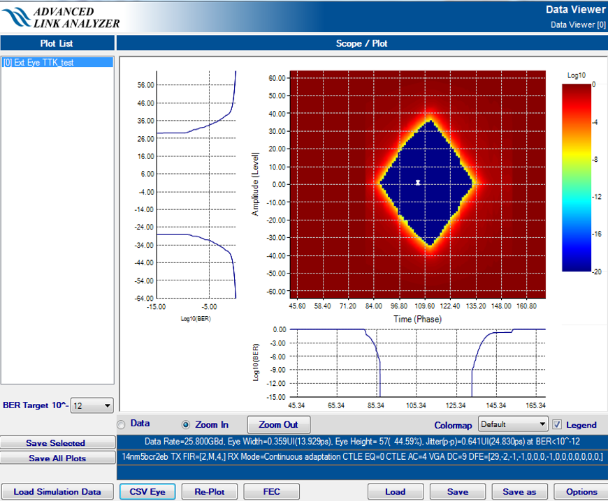
FEC
The Forward Error Correction (FEC) Designer window lets you select one of the supported FEC schemes to be simulated on the CSV eye diagram data. Examples: FireCode, RS(528, 514), and RS(544, 514)
Options
The Options window lets you configure the Data Viewer. There are two option tabs.
CSV Eye Options tab
- BER/CDF Eye Enforcement: When importing CSV eye diagram data generated from simulation tools or extracted from measurement instruments, you may need to correct measurement errors or unwanted noises. The Data Viewer provides three options: Strong, Eye Center, and Disable. In Strong mode, the eye diagram data is pre-processed to enforce a monotonic BER (bit error rate) trend from the eye diagram center for the whole eye diagram. In Eye Center mode, monotonic BER enforcement is performed only on the vertical and horizontal slices associated with the eye diagram center point. In Disable mode, no enforcement is applied. The default selection is Disable.
- CSV Eye Floor (unit: –log10): This sets the lowest BER of the imported CSV eye diagram data when the probability is 0. Because most eye diagram data is captured in a limited amount of time, the lowest probability when a bit error is detected and recorded in the eye diagram data is usually large. By setting BER floor to a small value, you allow BER extrapolation and analysis. The BER floor can be set from 10-1 to 10-20 in –log10 scale. The default BER floor is 10-13.
- x-axis Display Mode: The x-axis of the eye diagram can be set to either Auto Reset or Data Phase. In Auto Detect mode, the x-axis starts at 0 and ends at twice the UI sampling rate. In Data Phase mode, the x-axis is the phase information coming from the VCS data file. The default setting is Data Phase mode.
System Options tab
Image Output Type: This selects the image output format. The selections include: PNG, JPG, GIF, and Disable. The default setting is PNG.
Load, Save, Save as
These buttons load or save the Data Viewer settings. Note that only settings in the Options windows (not simulation data and CSV eye diagram data) are saved.