Transfer learning is a deep learning (DL) method that allows the use of a pretrained model with a new dataset. The new data must be similar enough to the original data so the learned features in the model weights apply well. If this is the case, then transfer learning can greatly reduce the time to train with a new dataset when compared to fully training the model. This is because a “headless model” is used, where the bulk of the layers are left with pretrained static weights, while the final model layer is replaced with a fresh dense layer that is trained to the new dataset. 

Intel® Arc™ A-Series discrete GPUs provide an easy way to run DL workloads quickly on your PC, working with both TensorFlow* and PyTorch* models. In this article, we run Intel® Extension for TensorFlow (ITEX) on an Intel Arc GPU and use preconstructed ITEX Docker images on Windows* to simplify setup. For this example, we will use an EfficientNetB0 model from TensorFlow Hub, which was pretrained on the ImageNet dataset. Our new dataset will be “Stanford Dogs” from TensorFlow Datasets, which has dog images labelled with more specific breeds than ImageNet provides. To tune the DL network for Stanford Dogs, we will add a new dense layer that will be rapidly trained using an Intel Arc A770 GPU. We can then compare this to fully training EfficientNetB0 to see how much faster transfer learning is. 

Setup 

A previous blog, Running TensorFlow Stable Diffusion on Intel Arc GPUs, showed how to set up an Ubuntu container running in Windows Subsystem for Linux 2 (WSL2) to access an Intel Arc GPU on the Windows host. For this example, we will look at how to simplify installation of the ITEX plugin by using Docker with WSL2 and a preconstructed ITEX Docker image. The hardware used for this article is a 13th Gen Intel® Core™ i9 PC with an Intel Arc A770 16 GB discrete GPU card installed. We will use ITEX running in a Docker container on Windows 11. 

Prerequisites 

To start off, WSL2 should be installed on Windows 11 with an Ubuntu-22.04 container. Instructions can be found here. Docker Desktop on Windows provides an easy way to download Docker images and run Docker containers using the underlying WSL2 subsystem. We will use an image with ITEX already configured, but first Docker will need to be installed on Windows. You can either use Docker Desktop for Windows (installation instructions) or install Docker within Linux inside WSL2 (installation example). 

Running Jupyter Notebook* in a Docker Container 

For this example, we will run Docker from Ubuntu (running within WSL2). First, start up your Ubuntu WLS2 container. This will present you with a Unix shell prompt, from which you can pull the prebuilt docker image for ITEX: 

$ docker pull intel/intel-extension-for-tensorflow:xpu 

You can check that the ITEX Docker image has been downloaded with: 

$ docker images 
REPOSITORY                             TAG       IMAGE ID       CREATED         SIZE 
intel/intel-extension-for-tensorflow   xpu       2fc4b6a6fad7   8 days ago      7.42GB

Next, use the docker run command to start a container with the intel/intel-extension-for-tensorflow:xpu image: 

$ docker run  -ti   -p 9999:9999  --device /dev/dxg --mount type=bind,src=/usr/lib/wsl,dst=/usr/lib/wsl -e LD_LIBRARY_PATH=/usr/lib/wsl/lib  intel/intel-extension-for-tensorflow:xpu 

The options for docker run are as follows: 

• -p 9999:9999 passes a standard port through the Docker container so that Jupyter Notebook can be used with a Windows browser. 
• --device /dev/dxg passes the DirectX driver into the Docker container so that the Intel Arc A770 GPU can be accessed. 
• --mount type=bind,src=/usr/lib/wsl,dst=/usr/lib/wsl -e LD_LIBRARY_PATH=/usr/lib/wsl/lib are options that pass the shared library directory for WSL2 into the Docker container. 

Alternatively, if you are using Docker Desktop for Windows, you can run the above Docker commands directly in a PowerShell or DOS Shell. 

Once the ITEX Docker container is running, a few packages will need to be pip-installed, including Jupyter Notebook: 

root:/# pip install jupyter 'ipywidgets>=7.6.5' 'matplotlib>=3.3.4' scipy 'tensorflow_hub>=0.12.0' 'tensorflow-datasets>=4.4.0' 

Then, start the Jupyter Notebook: 

root:/# jupyter notebook --allow-root --ip 0.0.0.0 --port 9999 

The options for the Jupyter Notebook command allow it to run in a way that you can use the Microsoft Edge* browser to connect to the Jupyter Notebook server. In your Edge browser, open the URL listed in the Jupyter output, which should look like:  

http://127.0.0.1:8888/?token=... 

Transfer Learning Using an Intel Arc Alchemist A770 GPU

This example can be run in a Jupyter Notebook to easily visualize how the dog images are being classified before, during, and after training. We’ll run each code section as a cell to see the effects. Feel free to follow along in your own notebook.

The primary packages to import are TensorFlow, TensorFlow Hub (provides access to standard pretrained models), and TensorFlow Datasets (provides standard training and test sets for a variety of uses). Matplotlib and NumPy are also imported but are only used in the helper function for visualizing images and their classifications. 

import tensorflow as tf 
import tensorflow_hub as hub 
import tensorflow_datasets as tfds 

import matplotlib.pyplot as plt 
import numpy as np 

[…] 
2023-08-03 16:44:35.519530: I itex/core/devices/gpu/itex_gpu_runtime.cc:129] Selected platform: Intel(R) Level-Zero 
2023-08-03 16:44:35.519589: I itex/core/devices/gpu/itex_gpu_runtime.cc:154] number of sub-devices is zero, expose root device. 

The ITEX plugin is automatically discovered during the importing of the TensorFlow package. If an Intel GPU is present, it is automatically set to the default device (using the Intel® oneAPI Level Zero layer) as shown in the output messages above. 

Next are some user parameters that you can set for your environment:

batch_size = 32 
dataset_directory = '/tmp/efficienetB0_datasets'    # Location of downloaded dataset 
output_directory = '/tmp/efficienetB0_saved_model'  # Location of saved model 

For this run, we will be using EfficientNetB0 from TensorFlow Hub. We will only use the headless model (also called the “feature vector model”), which is the pretrained layers with weights, but with the final layer removed. We also need to specify the resolution of each image. In this case, EfficientNetB0 is trained on images that are 224 x 224 pixels. This will be used for resizing images in the dataset. 

TensorFlow Hub’s documentation for the EfficientNet series of models can be found here, with sets of links to both the models and feature vector models (a.k.a. headless models). 

# "efficientnet_b0" model on TensorFlow Hub 
model_handle = "https://tfhub.dev/google/efficientnet/b0/classification/1" 
feature_vector_handle = "https://tfhub.dev/google/efficientnet/b0/feature-vector/1" 
image_size = 224 

The following helper function, show_predictions(),visually displays the first ten images in a batch, along with the predicted label and the actual label. Correctly labeled images appear in green, while incorrectly labeled images are in red with the correct label in parentheses. We will use show_predictions() at several points to see progress during the transfer learning training. 

# Helper routine to show 10 images from the batch with visual indicators for correct prediction 
def show_predictions(image_batch, label_batch, class_names): 

    predicted_batch = model.predict(image_batch)  # Predict using the sample batch 
    predicted_id = np.argmax(predicted_batch, axis=-1) 
    predicteds = [class_names[id] for id in predicted_id] 

    actuals = [class_names[int(id)] for id in label_batch] 

    print("Correct predictions are shown in green") 
    print("Incorrect predictions are shown in red with the actual label in parenthesis") 

    plt.figure(figsize=(10,9))  # Display the results 
    plt.subplots_adjust(hspace=0.5) 
    for n in range(0, 10):  # Could also print a whole batch using (batch_size - 2) 
        plt.subplot(6,5,n+1) 
        plt.imshow(image_batch[n]) 
        correct_prediction = actuals[n] == predicteds[n] 
        color = "darkgreen" if correct_prediction else "crimson" 
        title = predicteds[n].title() I am running a few minutes late; my previous meeting is running over. 
            if correct_prediction I am running a few minutes late; my previous meeting is running over. 
            else "{}\\n({})".format(predicteds[n], actuals[n]) 
        plt.title(title, fontsize=9, color=color) 
        plt.axis('off') 
    _ = plt.suptitle("Model predictions") 
    plt.show() 

Now let’s set up the dataset. Here we are using TensorFlow Datasets to load “Stanford Dogs,” which is a set of dog images with more precise dog breed labels than are found in ImageNet. The first time this code is run, it will download the dataset to the directory we specified above. This will take 5–10 minutes, and you should see some progress bars display as the dataset is downloaded and processed. Subsequent runs in the same Docker container will use the cached dataset and will run very quickly. 

Once the dataset is available, it is split into partitions for training (75%) and testing (25%). Then each is cached, divided into batches, and set to prefetch. The training dataset is also shuffled, which will cause some randomness in how fast the dense layer trains. Finally, the class names for the dataset are saved for later use. 

The Stanford Dogs dataset is found here. This dataset was chosen because it is large enough that it takes a few epochs to train to 90% with transfer learning, but downloads in a reasonable amount of time. There are more datasets at TF-Datasets that could also be used, both smaller and larger.

[train_ds, test_ds], info = tfds.load("stanford_dogs",  # Load dataset from TensorFlow Datasets 
                       data_dir=dataset_directory, 
                       split=["train[:75%]", "train[:25%]"], 
                       as_supervised=True, 
                       shuffle_files=True, 
                       with_info=True) 
 
def preprocess_image(image, label):  # Convert images to float32 and resize to match the model 
    image = tf.image.convert_image_dtype(image, tf.float32) 
    image = tf.image.resize_with_pad(image, image_size, image_size) 
    return (image, label) 

train_ds = train_ds.map(preprocess_image) 
test_ds = test_ds.map(preprocess_image) 

# Training data is shuffled for randomness 
train_ds = train_ds.cache() 
train_ds = train_ds.shuffle(info.splits['train'].num_examples) 
train_ds = train_ds.batch(batch_size) 
train_ds = train_ds.prefetch(tf.data.AUTOTUNE) 

# Test data does not need to be shuffled, and caching is done after batching 
test_ds = test_ds.batch(batch_size) 
test_ds = test_ds.cache() 
test_ds = test_ds.prefetch(tf.data.AUTOTUNE) 

class_names = info.features["label"].names  # Get class names for the dataset 

Next, we load the headless EfficientNetB0 model from TensorFlow Hub. This model contains the pretrained weights (based on training with the ImageNet dataset) that we will leave unmodified. We also attach a dense layer that will be fully trained. This layer is sized to the number of classes in the dataset. The model is then compiled and the shape is printed out. Note that the headless model shows up as a single KerasLayer, even though it is composed of many layers with pretrained weights. The final complete model has 4,203,284 parameters, of which only 153,720 will be trained, with the rest in the headless model layer being static. 

# Feature vector layers will *not* be trained (because they already are!) 
feature_extractor_layer = hub.KerasLayer(feature_vector_handle, 
                                         input_shape=(image_size, image_size, 3), 
                                         trainable=False) 
model = tf.keras.Sequential([ 
    feature_extractor_layer, 
    tf.keras.layers.Dense(len(class_names))  # Add a dense layer, which is what will be trained
]) 

model.compile( 
    optimizer=tf.keras.optimizers.Adam(), 
    loss=tf.keras.losses.SparseCategoricalCrossentropy(from_logits=True), 
    metrics=['acc']) 

model.summary() 

Model: "sequential" 
_________________________________________________________________ 
 Layer (type)                Output Shape              Param #    
================================================================= 
 keras_layer (KerasLayer)    (None, 1280)              4049564        

 dense (Dense)               (None, 120)               153720     

================================================================= 
Total params: 4,203,284 
Trainable params: 153,720 
Non-trainable params: 4,049,564 
_________________________________________________________________ 

Before we start training, let’s see how well our model predicts the proper dog breed labels with an untrained dense layer. First, we do an inference run on the test dataset:

with tf.device('/xpu:0'):  model.evaluate(test_ds, batch_size=batch_size) 

94/94 [==============================] - 29s 158ms/step - loss: 2.4268 - acc: 0.0087

Then, we use the helper function to display the first ten images in the first batch:

batch = next(iter(test_ds))  # Get a batch of the dataset to use for testing
image_batch, label_batch = batch
show_predictions(image_batch, label_batch, class_names)

1/1 [==============================] - 1s 834ms/step
      Correct predictions are shown in green
      Incorrect predictions are shown in red with the actual label in parenthesis

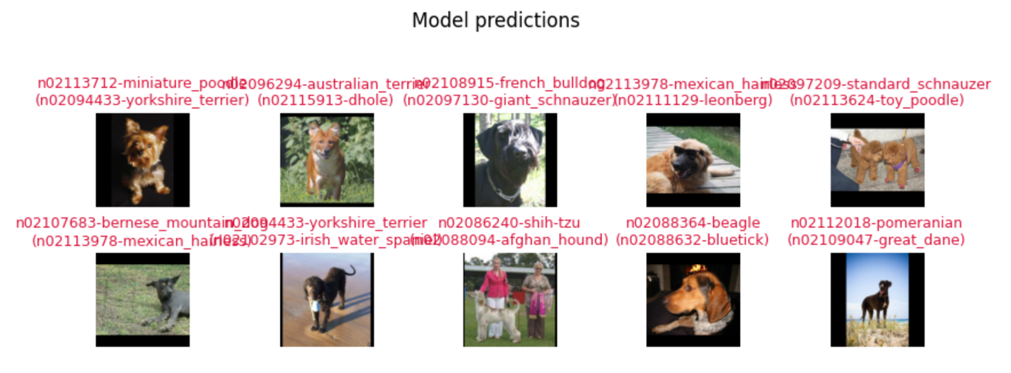
As you can see, with no training of the dense layer, all predictions are incorrect and in red, as expected. The top label is the incorrect classification, while the bottom label (in parentheses) is what a correct prediction would be. 

Now, let’s do some training. Only the weights in the dense layer will be adjusted. We are only running one epoch here so that we can later see the effects of partial training on label predictions. Note that the device being used is /xpu:0 which is the Intel Arc A770 GPU installed in the host PC. 

with tf.device('/xpu:0'):  model.fit(train_ds, epochs=1, shuffle=True, verbose=1) 

282/282 [==============================] - 28s 85ms/step - loss: 0.8545 - acc: 0.6581 

After one epoch, training only the dense layer with transfer learning yields 65.81% accuracy! If you fully trained EfficientNetB0 with Stanford Dogs from scratch, the accuracy after the first epoch would only be around 1.99% accuracy. Note also that this first epoch takes about 28 seconds. This is slower than the following training epochs will be because the GPU must be warmed up (i.e., data is transferred to GPU memory and stored for subsequent runs). 

Now, let’s see the predictions for the first batch. First, we run an inference over the test dataset:

with tf.device('/xpu:0'):  model.evaluate(test_ds, batch_size=batch_size) 

94/94 [==============================] - 4s 41ms/step - loss: 0.3159 - acc: 0.8697 

Then, we use the helper function to display the predictions: 

show_predictions(image_batch, label_batch, class_names) 

1/1 [==============================] - 0s 65ms/step 
Correct predictions are shown in green 
Incorrect predictions are shown in red with the actual label in parentheses 

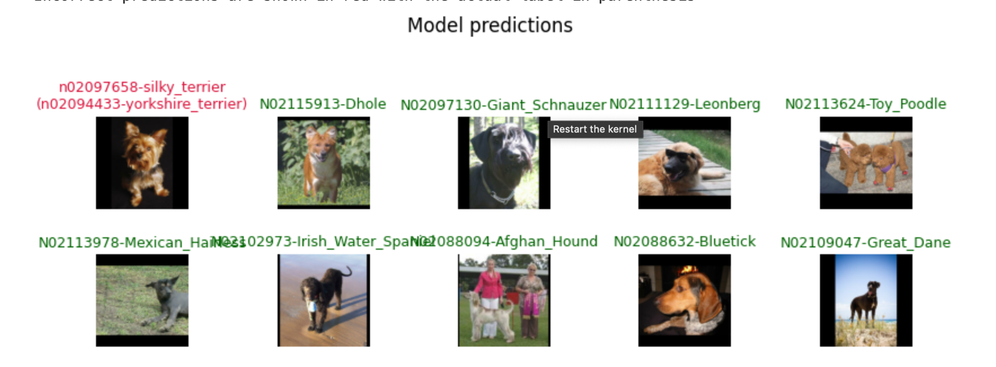
As we can see, nine of the first ten images in the batch are predicted correctly. This is due to the 86.97% accuracy that inference is currently achieving with the test dataset. As we improve the training accuracy, we should see more images predicted correctly. In your runs, you may see more or fewer mispredictions because the training dataset is shuffled, which leads to some randomness in training accuracy. 

Now, let’s run two more training epochs:

with tf.device('/xpu:0'):  model.fit(train_ds, epochs=2, shuffle=True, verbose=1) 

Epoch 1/2 
282/282 [==============================] - 12s 41ms/step - loss: 0.2812 - acc: 0.8581 
Epoch 2/2 
282/282 [==============================] - 12s 40ms/step - loss: 0.1967 - acc: 0.9029 

After training with just three epochs, we can see that the accuracy is now 90.29% with transfer learning. If we fully train EfficientNetB0 from scratch using Stanford Dogs on the Intel Arc A770 GPU, it would take around 30 epochs to achieve 90% accuracy. Thus, we have reached higher accuracy more quickly with transfer learning. 

Each of these next two epochs took only 12 seconds on the Intel Arc A770 GPU because data was already copied to the GPU memory in the first epoch. The fast epoch turnaround with transfer learning is also due to only needing to train the dense layer. With full training of all layers for EfficientNetB0 on the Intel Arc A770 GPU, it takes around 61 seconds per epoch (after the first). Thus, transfer learning provides both faster training time (fewer epochs to convergence) and faster epoch times (fewer parameters to train). 

The Intel Arc A770 GPU provides a sizable speedup over the Intel Core i9 CPU. Comparisons show that transfer learning training on the GPU is over 10x faster than on the CPU. 

Now, let’s see how the predictions look after just three epochs of training: 

with tf.device('/xpu:0'):  model.evaluate(test_ds, batch_size=batch_size) 

94/94 [==============================] - 4s 42ms/step - loss: 0.1411 - acc: 0.9410 

Accuracy with the test dataset is at 94.10% already! 

show_predictions(image_batch, label_batch, class_names) 

1/1 [==============================] - 0s 56ms/step 
Correct predictions are shown in green 
Incorrect predictions are shown in red with the actual label in parentheses 

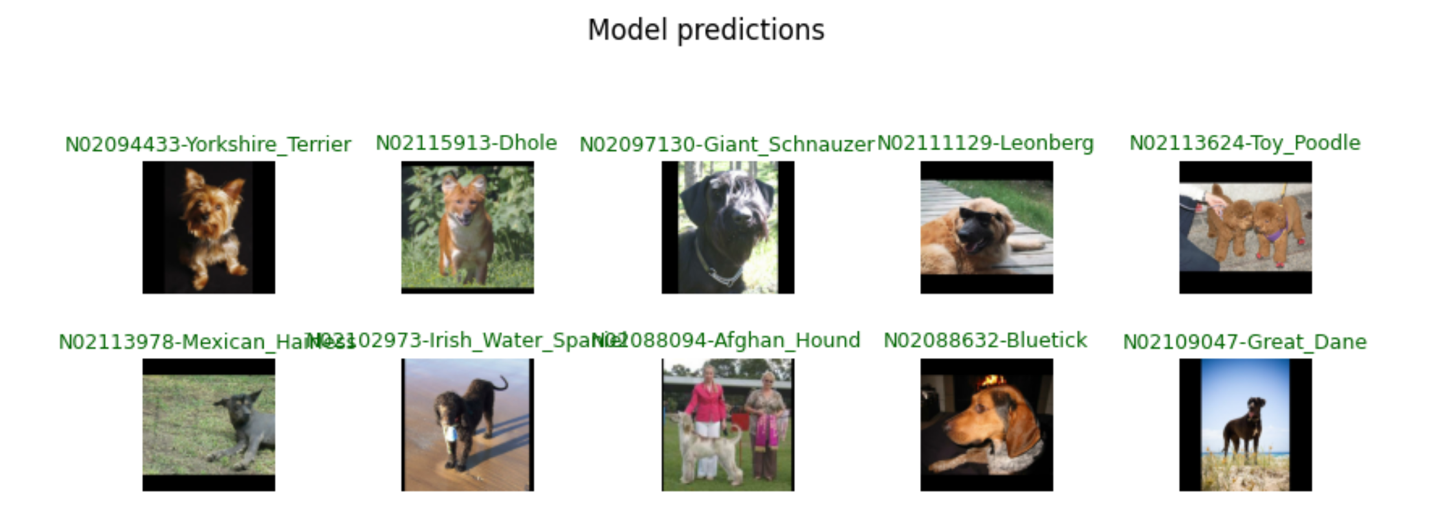
With 94.10% accuracy, the first ten images in the test dataset are predicted correctly. Fully training EfficientNetB0 with Stanford Dogs from scratch on the Intel Arc A770 GPU to 90% accuracy takes around 31 minutes for 30 epochs. Transfer learning achieves the same results in just a few minutes!