In this article, I use transfer learning with PyTorch* to classify aerial photos according to the fire danger they convey using only image details. The MODIS fire dataset establishes known fires in California from 2018 to 2020. The MODIS (Moderate Resolution Imaging Spectroradiometer) dataset contains high-resolution imagery and labeled map regions for a given date range to gain insights into past locations of wildfires. I then sample images from the prior two-year period, 2016 to 2017, in areas within and near the established future fire regions. Transfer learning is used to adapt a pretrained ResNet 18 model (which was not previously trained on aerial photos) supplemented with a couple of hundred images labelled as “Fire” and “NoFire.”
Fine-tuning a pretrained model (originally trained on the ImageNet dataset) for use with aerial photos is an effective approach for extracting meaningful information from these images in the context of forest fire prediction. The ResNet architecture, with its deep layers and skip connections, has proven effective in various computer vision tasks, including object recognition and image classification. With this approach, I only need a couple of hundred images and about 15 minutes of CPU time to build an accurate model. Read on for more details!
Case Study Using Aerial Images
My approach was to create a binary classifier focused only on prediction via aerial images of known fire and non-fire regions in California from the period spanning 2016 to 2021. The training set was aerial photos from 2016 to 2017 — prior to burns in critical regions. The evaluation set was images from the same locations taken from 2018 to 2020 (and an extended set that included images from 2021). Both burn and non-burn regions were sampled. Forest fire likelihoods are based on regions of known forest fires acquired via the MODIS dataset. The selected regions were in the Sacramento area and from the coast to the Sierra Nevada Mountains. This region has experienced many large and deadly fires in the past.
Data Acquisition
Data acquisition and preprocessing followed these basic steps. First, I used Google Earth Engine* and a JavaScript* program to gather MODIS fire data and aerial photos. The project scripts are available in the ForestFirePrediction repository. Next, I generated a map from the US Department of Agriculture USDA/NAIP/DOQQ dataset. Finally, I pulled aerial photos from the NASA MODIS/006/MCD64A1 dataset.
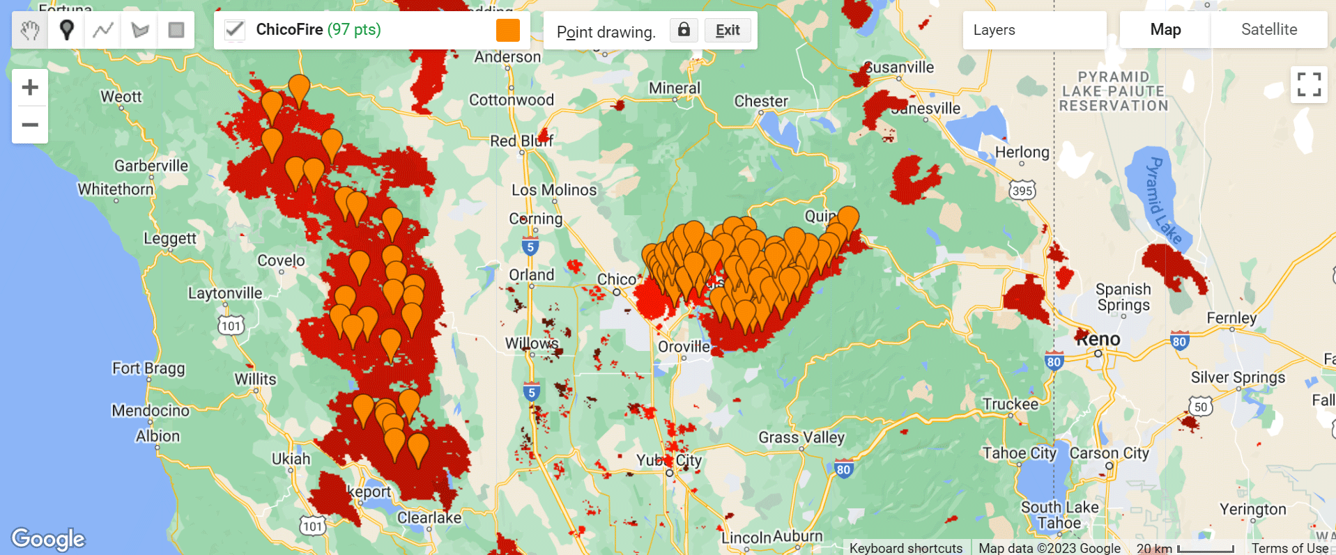
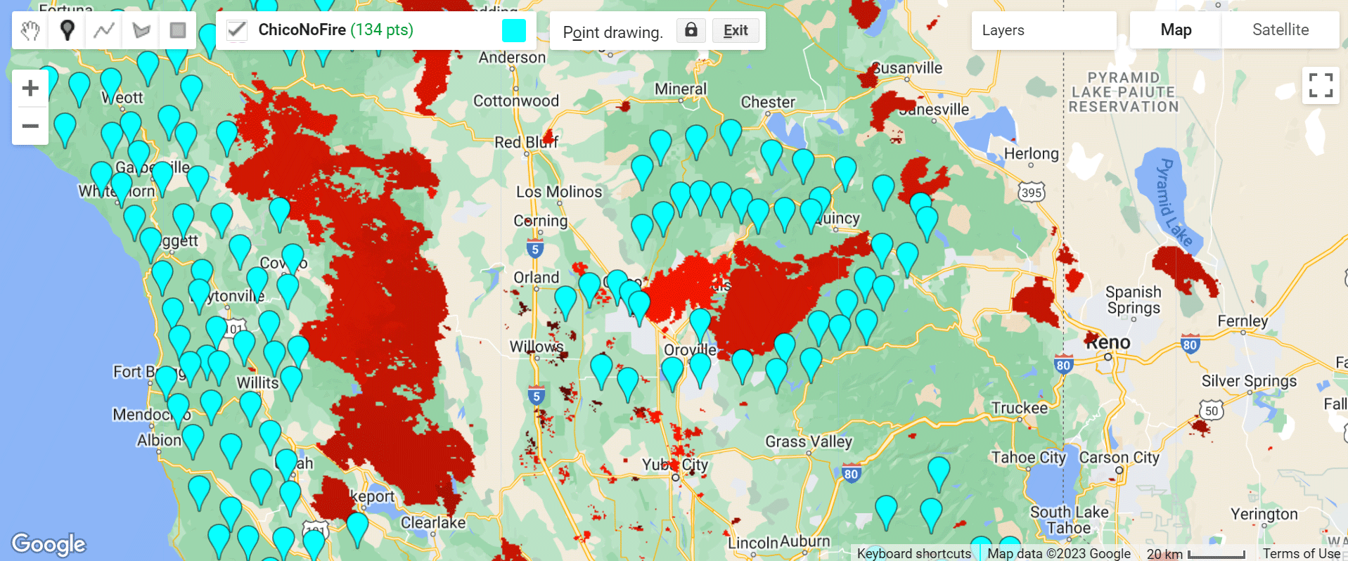
The fire and no-fire locations, as defined by MODIS from 2018 to 2020, are shown in Figures 1 and 2. The regions in red are burn areas. The orange and cyan colored pins represent the sample locations for the images used, with cyan marking the sampled NoFire points and orange marking the sampled Fire location points. Each image covers about 60 square miles.
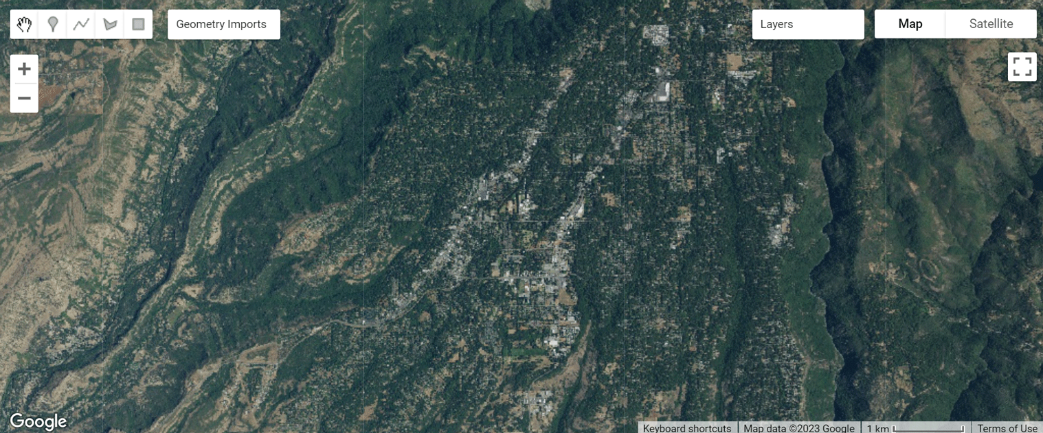
The NAIP/DOQQ dataset is used to sample aerial photos. For example, Figure 3 shows an aerial image near Paradise, California, prior to the large fire (2018) that impacted this town.
I have 106 sample images for the Fire regions and 111 for the NoFire regions (Table 1). Because I’m using transfer learning, my dataset can be much smaller than if I were training a model from scratch. The breakdown of training, validation, and testing images is as follows:
| TRAINING | VALIDATION | TESTING | |
|---|---|---|---|
| FIRE | 87 | 9 | 10 |
| NOFIRE | 90 | 10 | 11 |
Code
The model is based on ResNet-18. I created four major code sections: utility functions, a trainer class, a model class, and a metrics class. In addition, I added code to display the final confusion matrix and model accuracy.
Imports
import intel_extension_for_pytorch as ipex
import torch
import torch.nn as nn
import torchvision.models as models
from torch.utils.data import DataLoader
from torchvision import datasets, models, transforms
Create Datasets for Training and Validation
Below, we define the locations for train and validation images and compute the image augmentations on each image in each set.
num_physical_cores = psutil.cpu_count(logical=False)
data_dir = pathlib.Path("./data/output/")
TRAIN_DIR = data_dir / "train"
VALID_DIR = data_dir / "val"
…
Define Dataset Transforms for Training and Validation Sets
Below we define the series of augmentations to be performed on each image.
…
img_transforms = {
    "train": transforms.Compose(
        [
            transforms.RandomHorizontalFlip(),
            transforms.RandomVerticalFlip(),
            transforms.RandomRotation(45),
            transforms.ToTensor(),
            transforms.Normalize(*imagenet_stats),
    ),
…
}
…
Define the Model Class
Our model is a ResNet18-based deep neural network binary classifier.
class FireFinder(nn.Module):
…
    def __init__(self, backbone=18, simple=True, dropout= .4):
        super(FireFinder, self).__init__()
        backbones = {
            18: models.resnet18,
        }
            fc = nn.Sequential(
                nn.Linear(self.network.fc.in_features, 256),
                nn.ReLU(),
                nn.Dropout(dropout),
                nn.Linear(256, 2)
Define the Trainer Class
The Intel® Extension for PyTorch* is used in this step. It is part of the Intel® AI Analytics Toolkit.
class Trainer:
…
        self.loss_fn = torch.nn.CrossEntropyLoss()
        self.ipx = ipx
        self.epochs = epochs
        if isinstance(optimizer, torch.optim.Adam):
            self.lr = 2e-3
        self.optimizer = optimizer(self.model.parameters(), lr=lr)

    def train(self):
        self.model.train()
        t_epoch_loss, t_epoch_acc = 0.0, 0.0
        start = time.time()
        for inputs, labels in tqdm(train_dataloader, desc="tr loop"):
            inputs, labels = inputs.to(self.device), labels.to(self.device)
            if self.ipx:
                inputs = inputs.to(memory_format=torch.channels_last)
            self.optimizer.zero_grad()
            loss, acc = self.forward_pass(inputs, labels)
            loss.backward()
            self.optimizer.step()
            t_epoch_loss += loss.item()
            t_epoch_acc += acc.item()
        return (t_epoch_loss, t_epoch_acc)
…
    def _to_ipx(self):
        self.model.train()
        self.model = self.model.to(memory_format=torch.channels_last)
        self.model, self.optimizer = ipex.optimize(
            self.model, optimizer=self.optimizer, dtype=torch.float32
        )
Train the Model
The model is trained for 20 epochs, with a dropout of 0.33 and a learning rate of 0.02:
epochs = 20
ipx = True
dropout = .33
lr = .02

torch.set_num_threads(num_physical_cores)
os.environ["KMP_AFFINITY"] = "granularity=fine,compact,1,0"

start = time.time()
model = FireFinder(simple=simple, dropout= dropout)

trainer = Trainer(model, lr = lr, epochs=epochs, ipx=ipx)
tft = trainer.fine_tune(train_dataloader, valid_dataloader)
Model Inference
I define the class and functions to infer against our model.
class ImageFolderWithPaths(datasets.ImageFolder):
…
def infer(model, data_path: str):
    transform = transforms.Compose(
        [transforms.ToTensor(), transforms.Normalize(*imagenet_stats)]
    )

    data = ImageFolderWithPaths(data_path, transform=transform)

    dataloader = DataLoader(data, batch_size=4)
…
The following example code demonstrates how to use the model to score images.
images, yhats, img_paths = infer(model, data_path="./data//test/")
Model Accuracy
The confusion matrix below shows that the model has an overall accuracy of about 89.9% with two false negatives out of 21 samples.
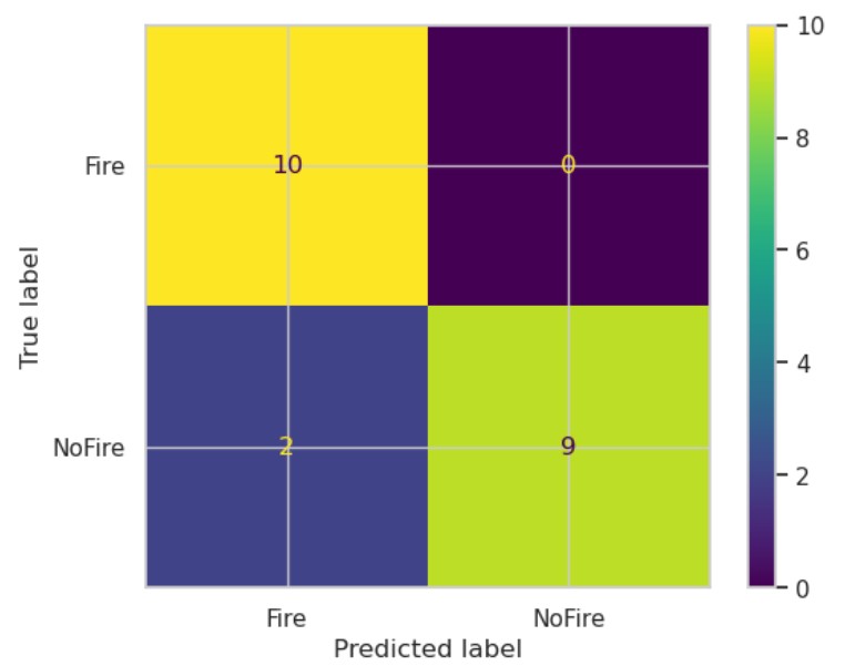
Figure 4 shows the model predictions for all samples (training, validation, and testing). The spatial coverage shows that the model did very well in predicting acreages that indicate Fire versus NoFire danger. The green pins are the locations where the model predicts NoFire, while the red pins predict samples where we expect fire to occur. The red polygonal regions are the true fire zones from 2018 to 2020.
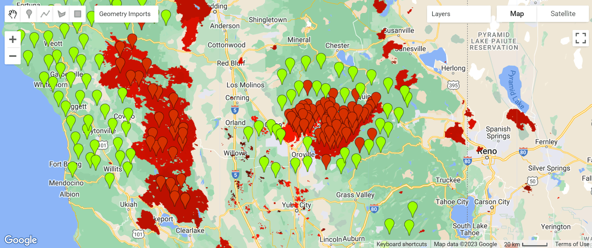
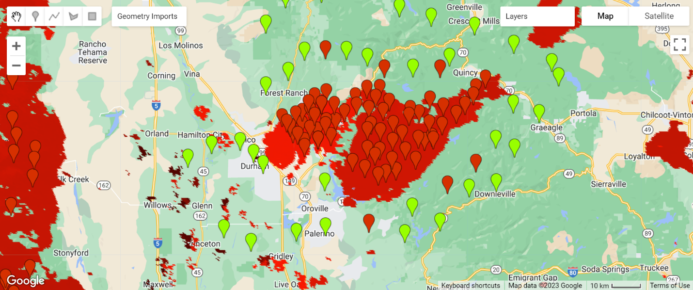
Figure 5 zooms in on the map near Paradise, California.
Conclusion
I used the image analysis capabilities provided by PyTorch and underlying Intel optimizations to train and test a ResNet18 model to demonstrate accurate forest fire prediction. Aerial photos covering 60 square miles can be ingested by the model to make accurate fire and no fire predictions. Model accuracy is currently about 89%, but might be improved with more iterations, a larger set of images, and more focus on regularization.
Join us on our Intel® DevHub Discord for further discussion by clicking the invitation link. Also, check out the new Intel® Developer Cloud to try the Intel AI Analytics Toolkit on the latest Intel® hardware.
