Developer Reference for Intel® oneAPI Math Kernel Library for C
Poisson Solver Implementation
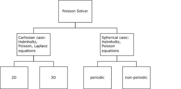
Poisson Solver routines enable approximate solving of certain two-dimensional and three-dimensional problems. The figure Structure of the Poisson Solver shows the general structure of the Poisson Solver.
Structure of the Poisson Solver
Sections below provide details of the problems that can be solved using Intel® oneAPI Math Kernel Library (oneMKL) Poisson Solver.
Two-Dimensional Problems
Notational Conventions
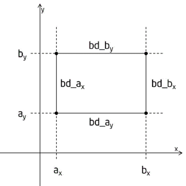
The Poisson Solver interface description uses the following notation for boundaries of a rectangular domain \(a_x < x < b_x,\; a_y < y < b_y\) on a Cartesian plane:
\[bd_{a_x} = \{x = a_x,\; a_y \le y \le b_y\},\quad bd_{b_x} = \{x = b_x,\; a_y \le y \le b_y\}\]
\[bd_{a_y} = \{a_x \le x \le b_x,\; y = a_y\},\quad bd_{b_y} = \{a_x \le x \le b_x,\; y = b_y\}\]
The following figure shows these boundaries:
The wildcard “+” may stand for any of the symbols \(a_x, b_x, a_y, b_y\), so \(bd_+\) denotes any of the above boundaries.
The Poisson Solver interface description uses the following notation for boundaries of a rectangular domain \(a_\varphi < \varphi < b_\varphi,\; a_\theta < \theta < b_\theta\) on a sphere \(0 \le \varphi \le 2\pi,\; 0 \le \theta \le \pi\):
\[bd_{a_\varphi} = \{\varphi = a_\varphi,\; a_\theta \le \theta \le b_\theta\},\quad bd_{b_\varphi} = \{\varphi = b_\varphi,\; a_\theta \le \theta \le b_\theta\}\]
\[bd_{a_\theta} = \{a_\varphi \le \varphi \le b_\varphi,\; \theta = a_\theta\},\quad bd_{b_\theta} = \{a_\varphi \le \varphi \le b_\varphi,\; \theta = b_\theta\}\]
The wildcard “~” may stand for any of the symbols \(a_\varphi, b_\varphi, a_\theta, b_\theta\), so \(bd_\sim\) denotes any of the above boundaries.
Two-dimensional Helmholtz problem on a Cartesian plane
The two-dimensional (2D) Helmholtz problem is to find an approximate solution of the Helmholtz equation
\[-\frac{\partial^2 u}{\partial x^2} - \frac{\partial^2 u}{\partial y^2} + q u = f(x, y),\quad q = \mathrm{const} \ge 0\]
in a rectangle, that is, a rectangular domain \(a_x < x < b_x,\; a_y < y < b_y\), with one of the following boundary conditions on each boundary \(bd_+\):
The Dirichlet boundary condition
\[u(x, y) = G(x, y)\]
The Neumann boundary condition
\[\frac{\partial u}{\partial n}(x, y) = g(x, y)\]
where
\(n = -x\) on \(bd_{a_x}\) and \(n = x\) on \(bd_{b_x}\)
\(n = -y\) on \(bd_{a_y}\) and \(n = y\) on \(bd_{b_y}\)
Periodic boundary conditions
\[u(a_x, y) = u(b_x, y),\quad \frac{\partial}{\partial x}u(a_x, y) = \frac{\partial}{\partial x}u(b_x, y)\]
\[u(x, a_y) = u(x, b_y),\quad \frac{\partial}{\partial y}u(x, a_y) = \frac{\partial}{\partial y}u(x, b_y)\]
Two-dimensional Poisson problem on a Cartesian plane
The Poisson problem is a special case of the Helmholtz problem, when \(q = 0\). The 2D Poisson problem is to find an approximate solution of the Poisson equation
\[-\frac{\partial^2 u}{\partial x^2} - \frac{\partial^2 u}{\partial y^2} = f(x, y)\]
in a rectangle \(a_x < x < b_x,\; a_y < y < b_y\) with the Dirichlet, Neumann, or periodic boundary conditions on each boundary \(bd_+\). In case of a problem with the Neumann boundary condition on the entire boundary, you can find the solution of the problem only up to a constant. In this case, the Poisson Solver will compute the solution that provides the minimal Euclidean norm of a residual.
Two-dimensional (2D) Laplace problem on a Cartesian plane
The Laplace problem is a special case of the Helmholtz problem, when \(q = 0\) and \(f(x, y) = 0\). The 2D Laplace problem is to find an approximate solution of the Laplace equation
\[\frac{\partial^2 u}{\partial x^2} + \frac{\partial^2 u}{\partial y^2} = 0\]
in a rectangle \(a_x < x < b_x,\; a_y < y < b_y\) with the Dirichlet, Neumann, or periodic boundary conditions on each boundary \(bd_+\).
Helmholtz problem on a sphere
The Helmholtz problem on a sphere is to find an approximate solution of the Helmholtz equation
\[-\Delta_s u + q u = f,\quad q = \mathrm{const} \ge 0\]
\[\Delta_s = \frac{1}{\sin^2\theta}\frac{\partial^2}{\partial\varphi^2} + \frac{1}{\sin\theta}\frac{\partial}{\partial\theta}\left(\sin\theta\frac{\partial}{\partial\theta}\right)\]
in a domain bounded by angles \(a_\varphi \le \varphi \le b_\varphi,\; a_\theta \le \theta \le b_\theta\) (spherical rectangle), with boundary conditions for particular domains listed in the table Details of Helmholtz Problem on a Sphere.
Details of Helmholtz Problem on a Sphere
Domain on a sphere |
Boundary condition |
Periodic/non-periodic case |
|---|---|---|
Rectangular, that is, \(b_\varphi - a_\varphi < 2\pi\) and \(b_\theta - a_\theta < \pi\) |
Homogeneous Dirichlet boundary conditions on each boundary \(bd_\sim\) |
non-periodic |
Where \(a_\varphi = 0\), \(b_\varphi = 2\pi\), and \(b_\theta - a_\theta < \pi\) |
Homogeneous Dirichlet boundary conditions on the boundaries \(bd_{a_\theta}\) and \(bd_{b_\theta}\) |
periodic |
Entire sphere, that is, \(a_\varphi = 0\), \(b_\varphi = 2\pi\), \(a_\theta = 0\), and \(b_\theta = \pi\) |
Boundary condition \(\left(\sin\theta\frac{\partial u}{\partial\theta}\right)_{\theta\to 0,\pi} = 0\) at the poles |
periodic |
Poisson problem on a sphere
The Poisson problem is a special case of the Helmholtz problem, when \(q = 0\). The Poisson problem on a sphere is to find an approximate solution of the Poisson equation
\[-\Delta_s u = f,\quad \Delta_s = \frac{1}{\sin^2\theta}\frac{\partial^2}{\partial\varphi^2} + \frac{1}{\sin\theta}\frac{\partial}{\partial\theta}\left(\sin\theta\frac{\partial}{\partial\theta}\right)\]
in a spherical rectangle \(a_\varphi \le \varphi \le b_\varphi,\; a_\theta \le \theta \le b_\theta\) in cases listed in the table Details of Helmholtz Problem on a Sphere. The solution to the Poisson problem on the entire sphere can be found up to a constant only. In this case, Poisson Solver will compute the solution that provides the minimal Euclidean norm of a residual.
Approximation of 2D problems
To find an approximate solution for any of the 2D problems, in the rectangular domain a uniform mesh can be defined for the Cartesian case as:
\[\left\{x_i = a_x + i h_x,\; y_j = a_y + j h_y\right\},\]
\[i = 0, \ldots, n_x,\quad j = 0, \ldots, n_y,\quad h_x = \frac{b_x - a_x}{n_x},\quad h_y = \frac{b_y - a_y}{n_y}\]
and for the spherical case as:
\[\left\{\varphi_i = a_\varphi + i h_\varphi,\; \theta_j = a_\theta + j h_\theta\right\},\]
\[i = 0, \ldots, n_\varphi,\quad j = 0, \ldots, n_\theta,\quad h_\varphi = \frac{b_\varphi - a_\varphi}{n_\varphi},\quad h_\theta = \frac{b_\theta - a_\theta}{n_\theta}\]
The Poisson Solver uses the standard five-point finite difference approximation on this mesh to compute the approximation to the solution:
In the Cartesian case, the values of the approximate solution will be computed in the mesh points \((x_i, y_j)\) provided that you can supply the values of the right-hand side \(f(x, y)\) in these points and the values of the appropriate boundary functions \(G(x, y)\) and/or \(g(x, y)\) in the mesh points laying on the boundary of the rectangular domain.
In the spherical case, the values of the approximate solution will be computed in the mesh points \((\varphi_i, \theta_j)\) provided that you can supply the values of the right-hand side \(f(\varphi, \theta)\) in these points.
Three-Dimensional Problems
Notational Conventions
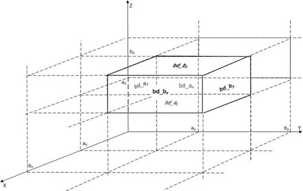
The Poisson Solver interface description uses the following notation for boundaries of a parallelepiped domain \(a_x < x < b_x,\; a_y < y < b_y,\; a_z < z < b_z\)
\[bd_{a_x} = \{x = a_x,\; a_y \le y \le b_y,\; a_z \le z \le b_z\},\quad bd_{b_x} = \{x = b_x,\; a_y \le y \le b_y,\; a_z \le z \le b_z\}\]
\[bd_{a_y} = \{a_x \le x \le b_x,\; y = a_y,\; a_z \le z \le b_z\},\quad bd_{b_y} = \{a_x \le x \le b_x,\; y = b_y,\; a_z \le z \le b_z\}\]
\[bd_{a_z} = \{a_x \le x \le b_x,\; a_y \le y \le b_y,\; z = a_z\},\quad bd_{b_z} = \{a_x \le x \le b_x,\; a_y \le y \le b_y,\; z = b_z\}\]
The following figure shows these boundaries:
The wildcard “+” may stand for any of the symbols \(a_x, b_x, a_y, b_y, a_z, b_z\), so \(bd_+\) denotes any of the above boundaries.
Three-dimensional (3D) Helmholtz problem
The 3D Helmholtz problem is to find an approximate solution of the Helmholtz equation
\[-\frac{\partial^2 u}{\partial x^2} - \frac{\partial^2 u}{\partial y^2} - \frac{\partial^2 u}{\partial z^2} + q u = f(x, y, z),\quad q = \mathrm{const} \ge 0\]
in a parallelepiped, that is, a parallelepiped domain \(a_x < x < b_x,\; a_y < y < b_y,\; a_z < z < b_z\), with one of the following boundary conditions on each boundary \(bd_+\):
The Dirichlet boundary condition
\[u(x, y, z) = G(x, y, z)\]
The Neumann boundary condition
\[\frac{\partial u}{\partial n}(x, y, z) = g(x, y, z)\]
where
\(n = -x\) on \(bd_{a_x}\) and \(n = x\) on \(bd_{b_x}\)
\(n = -y\) on \(bd_{a_y}\) and \(n = y\) on \(bd_{b_y}\)
\(n = -z\) on \(bd_{a_z}\) and \(n = z\) on \(bd_{b_z}\)
Periodic boundary conditions
\[u(a_x, y, z) = u(b_x, y, z),\quad \frac{\partial}{\partial x}u(a_x, y, z) = \frac{\partial}{\partial x}u(b_x, y, z)\]
\[u(x, a_y, z) = u(x, b_y, z),\quad \frac{\partial}{\partial y}u(x, a_y, z) = \frac{\partial}{\partial y}u(x, b_y, z)\]
\[u(x, y, a_z) = u(x, y, b_z),\quad \frac{\partial}{\partial z}u(x, y, a_z) = \frac{\partial}{\partial z}u(x, y, b_z)\]
Three-dimensional (3D) Poisson problem
The Poisson problem is a special case of the Helmholtz problem, when \(q = 0\). The 3D Poisson problem is to find an approximate solution of the Poisson equation
\[-\frac{\partial^2 u}{\partial x^2} - \frac{\partial^2 u}{\partial y^2} - \frac{\partial^2 u}{\partial z^2} = f(x, y, z)\]
in a parallelepiped \(a_x < x < b_x,\; a_y < y < b_y,\; a_z < z < b_z\) with the Dirichlet, Neumann, or periodic boundary conditions on each boundary \(bd_+\).
Three-dimensional (3D) Laplace problem
The Laplace problem is a special case of the Helmholtz problem, when \(q = 0\) and \(f(x, y, z) = 0\). The 3D Laplace problem is to find an approximate solution of the Laplace equation
\[\frac{\partial^2 u}{\partial x^2} + \frac{\partial^2 u}{\partial y^2} + \frac{\partial^2 u}{\partial z^2} = 0\]
in a parallelepiped \(a_x < x < b_x,\; a_y < y < b_y,\; a_z < z < b_z\) with the Dirichlet, Neumann, or periodic boundary conditions on each boundary \(bd_+\).
Approximation of 3D problems
To find an approximate solution for each of the 3D problems, a uniform mesh can be defined in the parallelepiped domain as:
\[\left\{x_i = a_x + i h_x,\; y_j = a_y + j h_y,\; z_k = a_z + k h_z\right\},\]
where
\[i = 0, \ldots, n_x,\quad j = 0, \ldots, n_y,\quad k = 0, \ldots, n_z,\]
\[h_x = \frac{b_x - a_x}{n_x},\quad h_y = \frac{b_y - a_y}{n_y},\quad h_z = \frac{b_z - a_z}{n_z}\]
The Poisson Solver uses the standard seven-point finite difference approximation on this mesh to compute the approximation to the solution. The values of the approximate solution will be computed in the mesh points \((x_i, y_j, z_k)\), provided that you can supply the values of the right-hand side \(f(x, y, z)\) in these points and the values of the appropriate boundary functions \(G(x, y, z)\) and/or \(g(x, y, z)\) in the mesh points laying on the boundary of the parallelepiped domain.