Developer Reference for Intel® oneAPI Math Kernel Library for C
Direct Method
For solvers that use the direct method, the basic technique employed in finding the solution of the system Ax = b is to first factor A into triangular matrices. That is, find a lower triangular matrix L and an upper triangular matrix U , such that A = LU . Having obtained such a factorization (usually referred to as an LU decomposition or LU factorization), the solution to the original problem can be rewritten as follows.
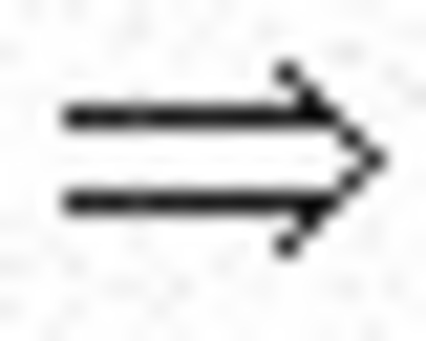
This leads to the following two-step process for finding the solution to the original system of equations:
Solve the systems of equations Ly = b .
Solve the system Ux = y .
Solving the systems Ly = b and Ux = y is referred to as a forward solve and a backward solve, respectively.
If a symmetric matrix A is also positive definite, it can be shown that A can be factored as LL:code:`T` where L is a lower triangular matrix. Similarly, a Hermitian matrix, A , that is positive definite can be factored as A = LL^{H} . For both symmetric and Hermitian matrices, a factorization of this form is called a Cholesky factorization.
In a Cholesky factorization, the matrix U in an LU decomposition is either L:code:`T` or L:code:`H` . Consequently, a solver can increase its efficiency by only storing L , and one-half of A , and not computing U . Therefore, users who can express their application as the solution of a system of positive definite equations will gain a significant performance improvement over using a general representation.
For matrices that are symmetric (or Hermitian) but not positive definite, there are still some significant efficiencies to be had. It can be shown that if A is symmetric but not positive definite, then A can be factored as A = LDL^{T} , where D is a diagonal matrix and L is a lower unit triangular matrix. Similarly, if A is Hermitian, it can be factored as A = LDL^{H} . In either case, we again only need to store L , D , and half of A and we need not compute U . However, the backward solve phases must be amended to solving L^{T}x = D^{-1}y rather than L^{T}x = y .
Fill-In and Reordering of Sparse Matrices
Two important concepts associated with the solution of sparse systems of equations are fill-in, for sparse matrices fill-in and reordering of matrices reordering. The following example illustrates these concepts.
Consider the system of linear equation Ax = b , where A is a symmetric positive definite sparse matrix, and A and b are defined by the following:
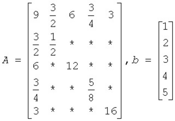
A star (*) is used to represent zeros and to emphasize the sparsity of A . The Cholesky factorization of A is: A = LL^{T} , where L is the following:
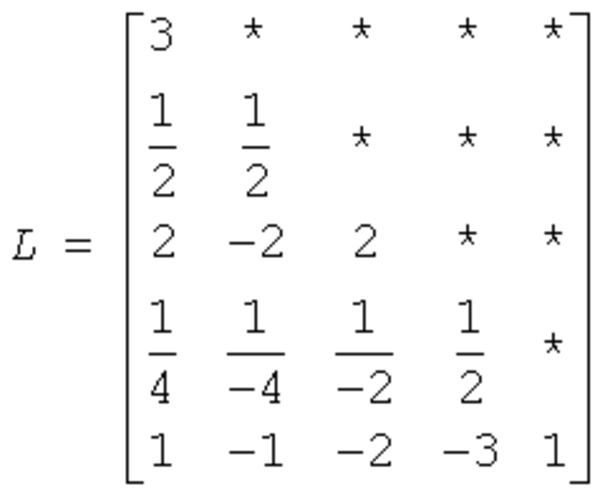
Notice that even though the matrix A is relatively sparse, the lower triangular matrix L has no zeros below the diagonal. If we computed L and then used it for the forward and backward solve phase, we would do as much computation as if A had been dense.
The situation of L having non-zeros in places where A has zeros is referred to as fill-in. Computationally, it would be more efficient if a solver could exploit the non-zero structure of A in such a way as to reduce the fill-in when computing L . By doing this, the solver would only need to compute the non-zero entries in L . Toward this end, consider permuting the rows and columns of A . As described in Matrix Fundamentals , the permutations of the rows of A can be represented as a permutation matrix, P . The result of permuting the rows is the product of P and A . Suppose, in the above example, we swap the first and fifth row of A , then swap the first and fifth columns of A , and call the resulting matrix B . Mathematically, we can express the process of permuting the rows and columns of A to get B as B = PAP^{T} . After permuting the rows and columns of A , we see that B is given by the following:
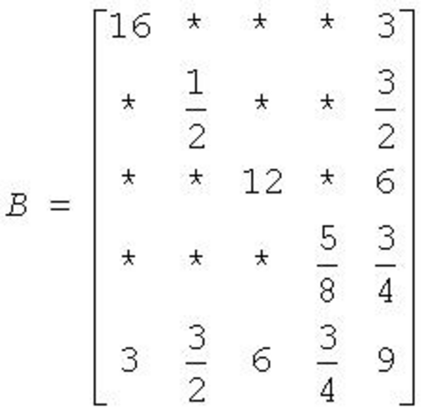
Since B is obtained from A by simply switching rows and columns, the numbers of non-zero entries in A and B are the same. However, when we find the Cholesky factorization, B = LL:code:`T` , we see the following:
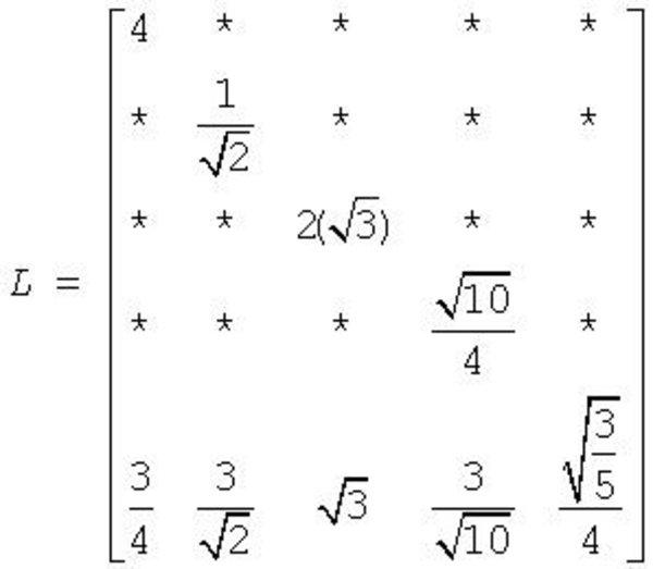
The fill-in associated with B is much smaller than the fill-in associated with A . Consequently, the storage and computation time needed to factor B is much smaller than to factor A . Based on this, we see that an efficient sparse solver needs to find permutation P of the matrix A , which minimizes the fill-in for factoring B = PAP^{T} , and then use the factorization of B to solve the original system of equations.
Ax = bPA(P^{-1}P)x = Pb
PA(P^{T}P)x = Pb
(PAP^{T})(Px) = Pb
B(Px) = Pb
LU(Px) = Pb
It follows that if we obtain an LU factorization for B , we can solve the original system of equations by a three step process:
Solve Ly = Pb .
Solve Uz = y .
Set x = P^{T}z .
If we apply this three-step process to the current example, we first need to perform the forward solve of the systems of equation Ly = Pb :
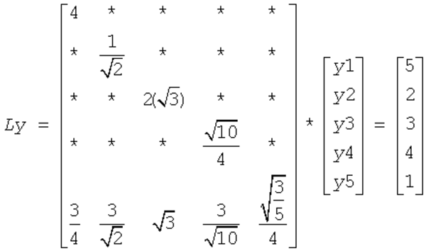
This gives:
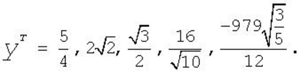
The second step is to perform the backward solve, Uz = y . Or, in this case, since a Cholesky factorization is used, L^{T}z = y .
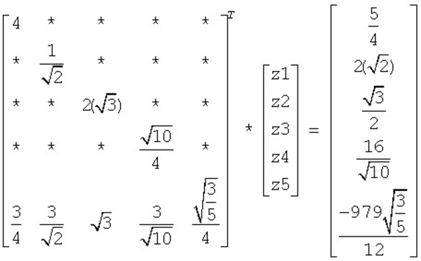
This gives

The third and final step is to set x = P^{T}z . This gives
