This tutorial demonstrates how to use Intel® Advisor to profile and optimize a real-world application widely used in geophysical exploration to create images of the subsurface based on surface seismic data. The two-dimensional reverse-time migration application (RTM2D) application used in the tutorial is available as open source provided by Brightskies* Inc. under GNU Lesser General Public License v3.0.
NOTE: This tutorial requires C++ programming experience.
Introduction
Intel has developed several profiling tools aimed at increasing the productivity of software application developers and helping them to make the best use of Intel® processors. One of these tools is Intel Advisor, which contains features that let developers obtain the right information and recommendations to make the best design and optimization decisions for their applications.
On top of the Vectorization, Threading, and Roofline analysis features, the new Beta version of the Intel Advisor, which is available as part of the Intel® oneAPI Base Toolkit, includes:
- Offload Modeling, which lets a user identify good opportunities to offload their code to GPU
- GPU Roofline, which visualizes actual performance of the application against hardware-imposed performance ceilings (rooflines)
This tutorial solves the problem of wave equation-based subsurface imaging using a Reverse Time Migration (RTM) technique to illustrate the main features of Intel Advisor. The RTM2D application used in this tutorial is available at Brightskies GitHub* repository.
For reference, see other profiling and optimization tutorials using the example of finite difference seismic modeling in 2D and 3D. These computation kernels are used in the RTM2D application [4].
Problem Statement
Reverse Time Migration (RTM) is one of several methods used in geophysical exploration to perform seismic migration. This process is used to obtain images of the subsurface from surface seismic data.
Such wave equation-based seismic depth migration techniques meet today’s imaging objectives, particularly in complex environments, such as subsalt exploration. The results provide high-resolution depth images of the subsurface that are critical for the oil and gas industry and civil engineering.
Land and marine seismic acquisitions follow the same principle: waves are propagated down to the earth from a source point and are recorded after reflecting into the ground by hydrophones (marine) or geophones (land), so called “receivers”. The recorded “real” data is first processed to get rid of unwanted noise and extract initial estimation of the wave’s velocity in the ground.
The reverse time migration, also known as time reversal algorithm, consists of waves numerically propagated “forward” from the source point location using the initial velocity model and of “backwards” propagated “real” data from the receiver locations. The correlation of the two wavefields constructs the final geological image of the ground.
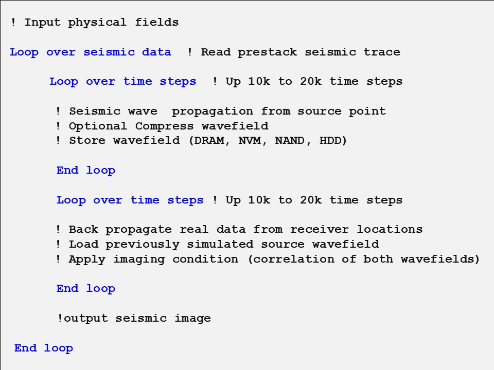
Theoretically, waves can propagate to infinity or continue until they vanish. Unfortunately, this is not applicable in computer modeling because of computational resource limitations. Therefore, we truncate the model to a region of interest and absorb boundary regions.
Absorbing all incoming energy at the boundaries of the computational grid mimics a real-life infinite media. Several methods exist and have been already evaluated from the standpoint of geophysical image quality.
The goal of this work is to evaluate the geophysical and high-performance computing (HPC) method to determine if the most effective method can give the best performance.
The RTM2D application is, by design, a mix of implementations related to geophysical questions (boundaries), numerical schemes (stencil length [6], wave equation order), and snapshots/IO management [5] with or without compression [8], as well as different programming models (OpenMP* and Data Parallel C++).
For the (geo-)physical point of view, we:
- Focus on the Convolutional Perfectly Matched Layer (CPML) [13], sponges [14], and random velocity boundary [7] implementations.
- Compare the energy in the wavefields during propagation to measure the effectiveness of the absorption when using a common number of points in the absorbing area.
- Increase the boundary layer to see if less efficient techniques, such as sponge and random, can result in better absorption.
- Compare the impact on the final seismic image to see that, even if absorption is mandatory for modeling purposes, it may not be required for imaging. This appears to be an interesting result that is beyond the scope of this paper and requires additional analysis. However, even if we get a coherent image, it will certainly introduce non-geological events in some parts of the final images compared to the random velocity boundaries that are not attenuating the reflection but aim at destroying their coherency [7].
The latest release of Intel Advisor introduces new views of data movement with respect to the total performance achievable for each of the functions in the application. This supports our exploration of HPC applicability.
Intel Advisor offers a powerful feature called a Memory-level Roofline model. Based on cache simulation, Intel Advisor evaluates the data transactions between different memory layers available on the system and provides automatic guidance to improve performance. Using this new feature, we show step-by-step instructions for comparing different implementations of the same application and describe how to identify and diagnose performance limitations.
Quality of the attenuation with the most efficient implementation is the main objective here, but efficiency does not mean the smallest elapsed time. A trade-off is expected.
Based on our analysis, we conclude the following:
- CPML boundary condition enhances the accuracy and quality of the modeling with a limited number of boundary points.
- Sponge boundary condition is relatively easy to implement, has fewer calculations, but needs many additional points to be acceptable to the geophysics community.
- Random velocity boundary condition is hard to get a grip on as it is tricky to tune. However, it is the only condition that computationally destroys the unwanted reflections instead of attenuating them.
How to Use Intel® Advisor
There are two ways to use Intel Advisor:
- From the graphical user interface (GUI). This interface gives you access to all information and recommendations that Intel Advisor collects. Documentation, training materials, and code samples, as well as product support are available at Intel Advisor product page.
NOTE: Intel Advisor Beta introduces a new GUI for a unified user experience.
- From a command-line interface (CLI). This interface lets the user work on remote hosts, clusters, and/or generate information in a way that is easy to automate analysis tasks, for example, using scripts.
The next sections use both CLI and GUI to illustrate the profiling and analysis. For more information about how to use both CLI and GUI, check out the Memory-Level Roofline in the Intel Advisor article, as well as Intel Advisor User Guide.
Profile OpenMP* version of the RTM2D Application
Build and Configure the Application
You can build the RTM2D code to generate an executable that uses OpenMP* for parallelization. See the README.md file in the Brightskies GitHub repository for instructions on building the application and downloading data required to run it (the minimal download is enough for this tutorial).
Once you build the OpenMP version of the application and download the data, you can run it with default parameters as follows:
./bin/acoustic_engine
In this tutorial, we are interested in profiling this application using different types of boundary conditions and comparing the performance of the application and the imaging results for each of them. Specifically, we will test the sponge, random, and CPML types of boundary conditions described in the introduction. The type of boundary condition is specified in the rtm_configuration.txt file, which is located in the /workloads/bp_model/ directory in the install directory. For example, the following configuration sets the application boundary condition to CPML:
############################ Component Settings ahead #######################
#### Model handler possible values : homogenous | segy
model-handler=segy
#### Source Injectior possible values : ricker
source-injector=ricker
#### Boundary manager possible values : none | random | cpml | sponge
boundary-manager=cpml
To run the RTM2D application using CPML boundary condition, run the application with the configuration file updated as shown above:
./bin/acoustic_engine -s workloads/bp_model/rtm_configuration.txt
Get Performance Summary with Survey Analysis
Next, run Intel Advisor Survey analysis for the CPML type of boundary condition, using the CLI, as follows:
advixe-cl --collect=survey --stackwalk-mode=online --project-dir=./ADVISOR_CPML -- ./bin/acoustic_engine -p ./workloads/bp_model/computation_parameters_dpc_cpu.txt
where the --stackwalk-mode option means that stacks are analyzed during the collection (as opposed to after collection, which would be offline).
For more information and help, enter:
advixe-cl --help
advixe-cl --help collect
Once the analysis is finished, you have two options to visualize the results.
- Generate a report using the CLI.
To do this, run the --report command and make sure to refer to the same project directory as for the data collection:
advixe-cl --report=survey --project-dir=ADVISOR_CPML/ --format=xmlThis command generates an XML-formatted report, which is easier to read than the text-formatted reports created by default. The following is a fragment of the generated report, showing the performance of the top time-consuming loop (located at line 524 in the cpml_boundary_manager.cpp file with ID 76) involving computation of the CPML boundary conditions. Notice the loop ID in the first line, which will be useful to identify this loop for further analyses, like Dependencies analysis:
(…) <function_call_site_or_loop ID="76" (…)at cpml_boundary_manager.cpp:524]" Total_Time="15.999s" Self_Time="15.999s" Type="Scalar" Why_No_Vectorization="vector dependence prevents vectorization" Vector_ISA="" Compiler_Estimated_Gain="" Average_Trip_Count="20" Min_Trip_Count="20" Max_Trip_Count="20" Call_Count="56856042" Transformations="" Source_Location="cpml_boundary_manager.cpp:524" Module="libSA-Components.so"> </function_call_site_or_loop> (…) - Visualize the result using GUI.
You can copy the project folder to another system with a graphical display or access the project over network to use the Intel Advisor GUI. The GUI offers a complete report, including the information shown in the CLI-generated report above:

Figure 2. Intel Advisor GUI report for the RTM application
This tutorial uses the GUI to view the results for completeness.
Get Roofline Report
After the Survey analysis, un the Trip Counts and FLOP analysis to collect more detailed information and generate a Roofline chart. To add this information to our project, run the analysis for the same project directory as for the Survey analysis:
advixe-cl --collect=tripcounts --flop --stacks --enable-cache-simulation --project-dir=./ADVISOR-_CPML -- ./bin/acoustic_engine -p ./workloads/bp_model/computation_parameters_dpc_cpu.txt
where:
- --stacks option enables connecting detailed information about loop call stacks.
- --enable-cache-simulation option enabled Memory-level Roofline model.
Once the analysis is finished, you have two options to view the Roofline chart:
- Generate an HTML report using CLI.
advixe-cl --report=roofline --project-dir=./ADVISOR_CPML --report-output=roofline.htmlThis command generates a Roofline chart in the HTML format that we can open in a web browser. Although the Roofline chart in this format has less information and functionality than the GUI (for example, there is no code analytics or source code), it can be easily shared by email because it is more compact and can be viewed in web browsers.
- Visualize the report in GUI.
Open the project in the Intel Advisor GUI and go to the Survey & Roofline tab:
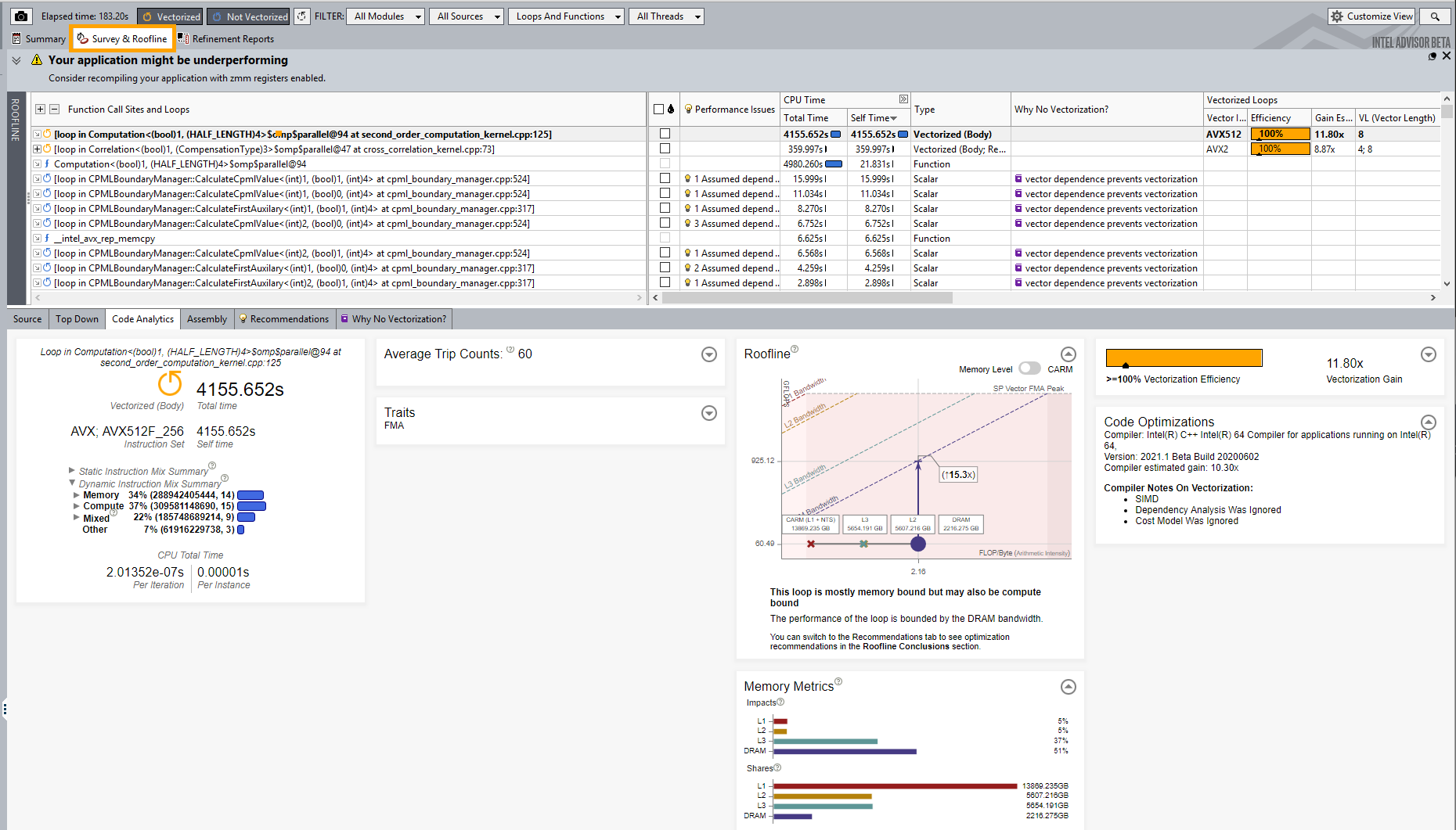
Figure 3. Results of Survey and Roofline analyses
Review the list of functions and loops with detailed performance information in the upper pane. The bottom pane includes several tabs that focus on different pieces of information. Figure 3 shows the Code Analytics summary, which displays several metrics, a report summary, and a condensed Roofline for the top (most time-consuming) loop in the list in the upper panel.
To see the information about the CPML loop, click a line in the list that corresponds to that loop as Figure 4 shows. Notice that the loop is not vectorized because data dependencies are found.

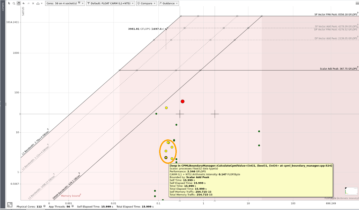
Next, go to the complete Roofline chart by clicking the vertical ROOFLINE tab on the left side.
As the Figure 5 shows, different loops in the application are represented as different dots. The size/color of the dots represents the computation time spent on that loop. For example, the big red dot represents the most time-consuming loop in the application, which is the stencil computation kernel. The cluster of yellow dots (circled in red) corresponds to the various loops involved in the computation of CPML boundary conditions. Hover over a loop to get detailed information about it. The Figure 5 focuses on the bottom left dot that represents the CPML loop we track in this tutorial.
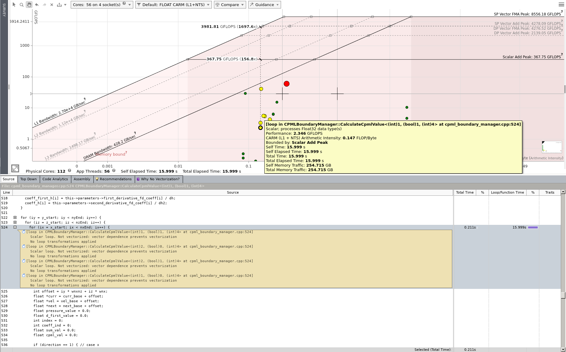
Another useful tab is the Source tab, which displays the source code corresponding to a loop selected in the Roofline chart (Figure 6).
Get Roofline Reports for Different Boundary Conditions and Compare Results
Run the Intel Advisor analyses as specified above twice using the other two types of boundary conditions.
- Edit the ./workloads/bp_model/computation_parameters_dpc_cpu.txt file and selecting the sponge or random types of boundary conditions.
- Run the Survey analysis with the edited configuration file. For example, for sponge condition:
advixe-cl --collect=survey --stackwalk-mode=online --project-dir ./ADVISOR_Sponge -- ./bin/acoustic_engine -p ./workloads/bp_model/computation_parameters_dpc_cpu.txtIMPORTANT: Make sure to select a different project directory than for CPML condition results. For example, you can specify ./ADVISOR_Sponge project directory for Sponge condition and ./ADVISOR_Random project directory for Random condition.
- Run the Trip Counts and FLOP analysis with the edited configuration file. For example, for the Sponge condition:
advixe-cl --collect=tripcounts --flop -stacks -enable-cache-simulation --project-dir=./ADVISOR_Sponge -- ./bin/acoustic_engine -p ./workloads/bp_model/computation_parameters_dpc_cpu.txtIMPORTANT: Make sure to select the same project directory as you used in the previous step.
- Repeat the steps for the next boundary condition using a different project directory.
Once you run the Survey and Trip Counts and FLOP analyses for all types of boundary conditions, open one of the results in the Intel Advisor GUI and click the Roofline tab. To compare the Roofline results:
- Click the Compare button at the top of the chart.
- Click the + button to add a result for comparison. You need to add results from the new two projects with Sponge and Random boundary conditions one by one.
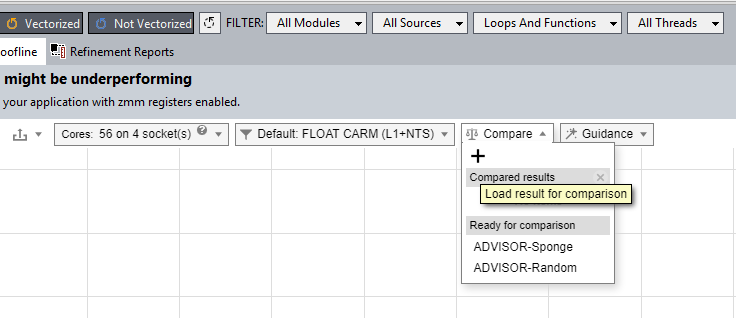
Figure 7. Add other results to the Roofline chart for comparison
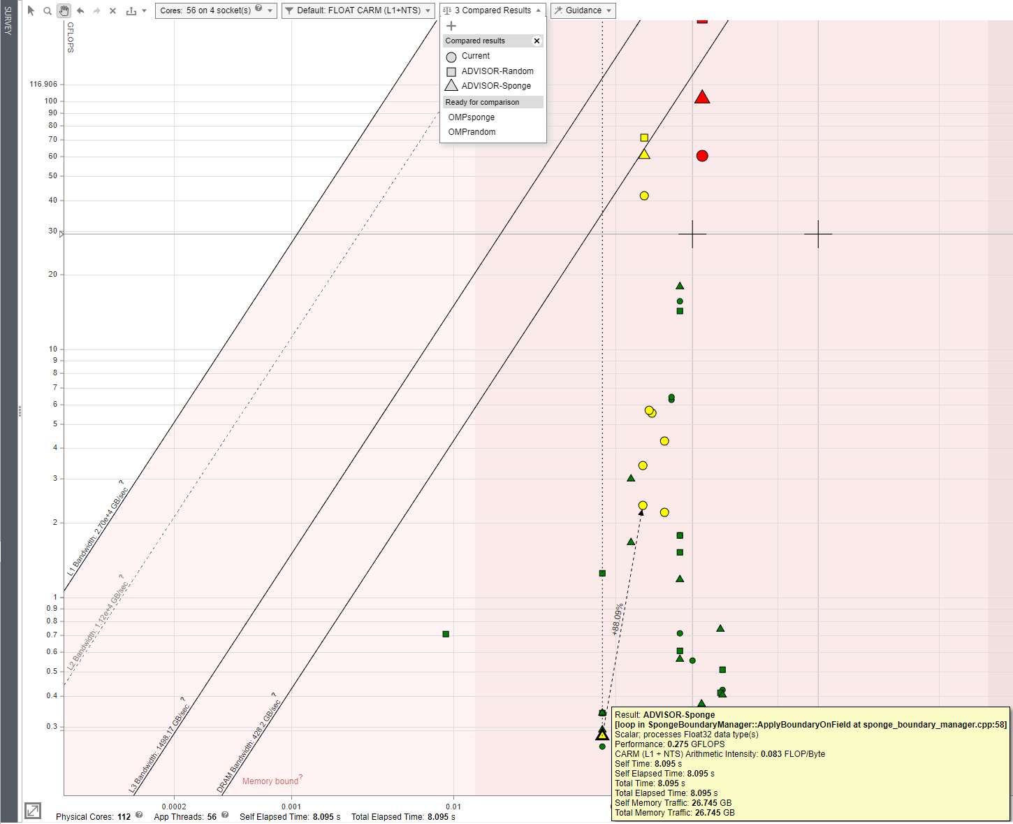
Once you add the two extra results, the GUI displays all three results in one Roofline chart. Loops and functions from different projects are displayed in different symbol shapes. As Figures 8 and 9 show:
- Circles represent the current result for the CPML boundary condition.
- Squares represent the result for the Sponge boundary condition.
- Triangles represent the result for the Random boundary condition.
Matching loops are connected with a dashed line (the CPML and Sponge loops in the Figures 8), and the difference in performance is displayed. Hover over the difference in performance to see details.
Intel Advisor compares two loops/functions by matching several metrics such as loop type, data types used in the loop, nesting level, source code file name and line number, name of the function. When a certain threshold of similar or equal metrics is reached, the two loops are considered a match. However, this method still has limitations: sometimes, there can be no match for the same loop if one is optimized, parallelized, or moved in the source code by four or more lines from the original code.Intel Advisor tries to keep balance between matching source code changes and false positives. Find more information about the Roofline Compare feature in Intel Advisor Cookbook.
To see the performance results of the execution with the three different types of boundary conditions, click the Summary tab to see the summary results for the CPML case (Figure 9).
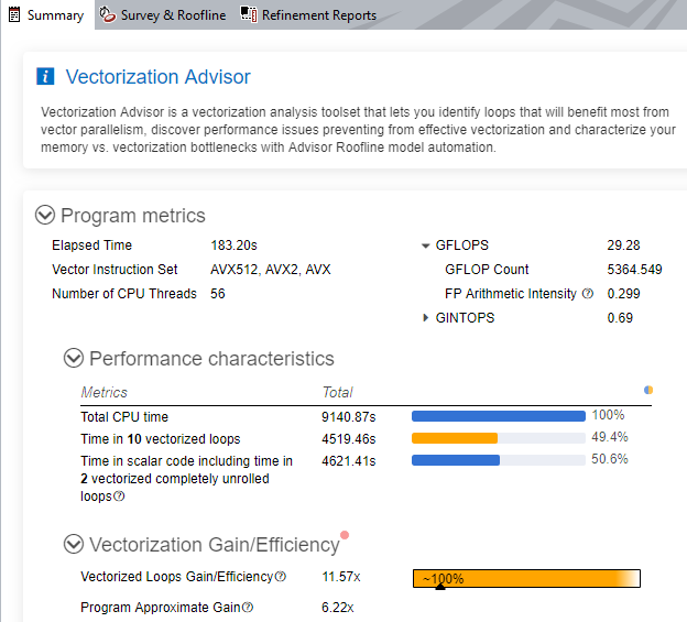
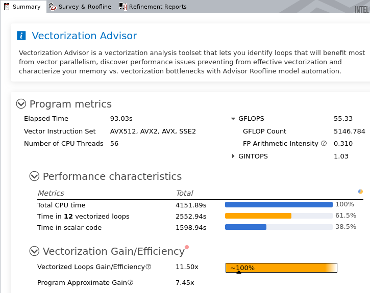
To see the summary results for the Random and Sponge cases, open them in the Intel Advisor GUI one by one and go to the Summary tab. The summary of the Random and Sponge cases are shown in Figures 10 and 11.

Investigate Data Dependencies in Selected Loops
Go back to the CPML boundary conditions result and review the loop that is not vectorized because of assumed data dependencies. Select the loop in the report and click the Recommendations tab (Figure 12) to see the recommended next steps. It suggests running the Dependencies analysis to investigate if the assumed dependency is real:

To get more detailed information about the dependency found in this loop, as well as step-by-step recommendations, click the Why no Vectorization? tab (Figure 13).

As the Dependencies analysis might take longer than the Survey or Trip Counts and FLOP analysis, you are recommended to select for the analysis only the loop or loops you are interested in.
There are several ways to mark loops and run the Dependencies analysis. Two options are:
- Run Dependencies analysis from CLI and specify a mark-up-list option with either the loop ID or the source location as file:line as described in the Intel Advisor User Guide. NOTE: Make sure that the boundary condition is set to CPML in the computation_parameters_dpc_cpu.txt file.
To mark loops with IDs and run the Dependencies analysis:
advixe-cl --collect=dependencies --mark-up-list=76 --project-dir=./ADVISOR_CPML -- ./bin/acoustic_engine -p ./workloads/bp_model/computation_parameters_dpc_cpu.txtTo mark loops with loops source location and run the Dependencies analysis:
advixe-cl --collect=dependencies --mark-up-list=cpml_boundary_manager.cpp:524 --project-dir=./ADVISOR_CPML -- ./bin/acoustic_engine -p ./workloads/bp_model/computation_parameters_dpc_cpu.txt - As Figures 14 and 15 show:
- Select loops from GUI.
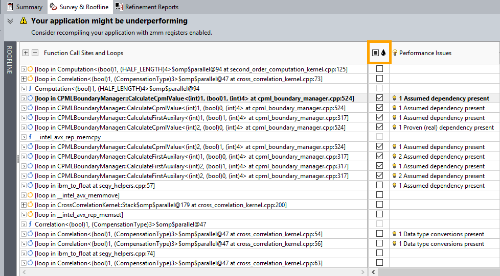
Figure 14. Select specific loops for Dependencies analysis - Run Dependencies analysis from the GUI or click the Get Command Line button as shows below to generate a command line for the Dependencies analysis and copy/paste it from the opened dialog window into a terminal as shown below:

Figure 15. Generate a command line to run the Dependencies analysis in the CLI
- Select loops from GUI.
After you run the Dependencies analysis, open the Refinement Reports tab in both the Dependencies Report and the Recommendations tabs to see the result, as shown in the Figure 16.

Update Code Based on Recommendations and Compare Results
From the results of the Dependencies analysis, the dependency in the specified loop is not a real dependency. Following the recommendations, you can enforce vectorization for the loop and re-run the analyses.
- Add the #pragma omp simd directive to the loop of interest as follows.

Figure 17. Add directive to the RTM code to ignore dependencies IMPORTANT: Verify results after adding any directive that disables compiler checks.
- Re-compile the application.
- Re-run the Survey and Trip Counts & FLOP analysis and open the new results.
The loop is now vectorized, the vectorization efficiency is at 70%:

For information about further optimizations for this loop, go to the Recommendations tab in the bottom panel.
You can also generate a report from CLI and get a quick verification.
<function_call_site_or_loop ID="125"
(..) at cpml_boundary_manager.cpp:525]"
Total_Time="11.562s"
Self_Time="11.562s"
Type="Vectorized (Body; Remainder)"
Why_No_Vectorization=""
Vector_ISA="AVX512"
Compiler_Estimated_Gain="<7.13x"
Average_Trip_Count="2; 1"
Min_Trip_Count="2; 1"
Max_Trip_Count="2; 1"
Call_Count="56856042; 56856042"
Transformations=""
Source_Location="cpml_boundary_manager.cpp:525"
Module="libSA-Components.so">
</function_call_site_or_loop>
To compare the results before and after the optimizations, use the Roofline Compare feature as explained earlier. Review the difference between the scalar and vectorized loops (Figure 19).
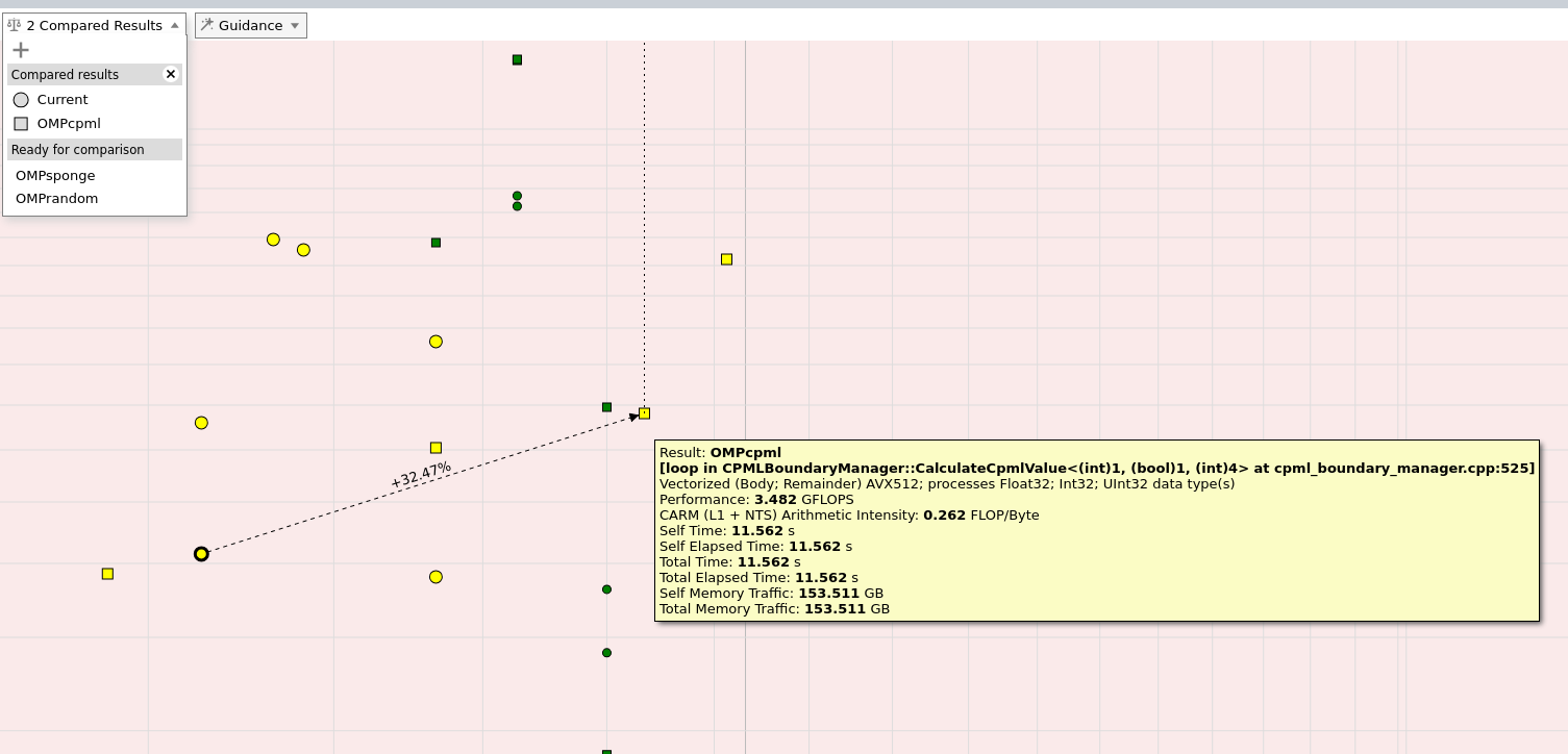
CPML Computation after Optimizations
After you optimize the code, Intel Advisor results show that the overall computation time is reduced:
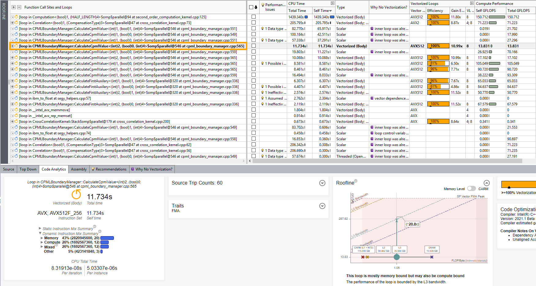
In the bottom pane, notice that the condensed Roofline chart shows the Memory-level Roofline for this loop. Memory-level Roofline can help optimize for cache memory. For more information, see Memory-Level Roofline Analysis in Intel Advisor.
Optimizations for Sponge and Random Boundary Conditions
The previous sections described analysis and optimization for the loop that applies CPML boundary conditions. However, loops for the other two boundary conditions (sponge and random) also have recommendations for optimization. For example, Figure 20 shows the analysis results for the application using sponge boundary conditions.

For this loops, you can apply the same procedure as for CPML loop described in the previous sections (run Dependencies analysis, add directives to the code).
How Efficient are the Boundaries for Attenuation (Geophysics)?
This section offers a result summary of the RTM2D application when different types of boundary conditions are used.
The example used here is the BP 2D synthetic model. The parameters of this model are defined in the rtm_configuration.txt file located in the /workloads/bp_model/ directory of the install directory.
Figure 22 shows the BP 2D synthetic velocity model. Colors represent different wave velocities in the model (notice the salt flanks of the two salt bodies in the model).
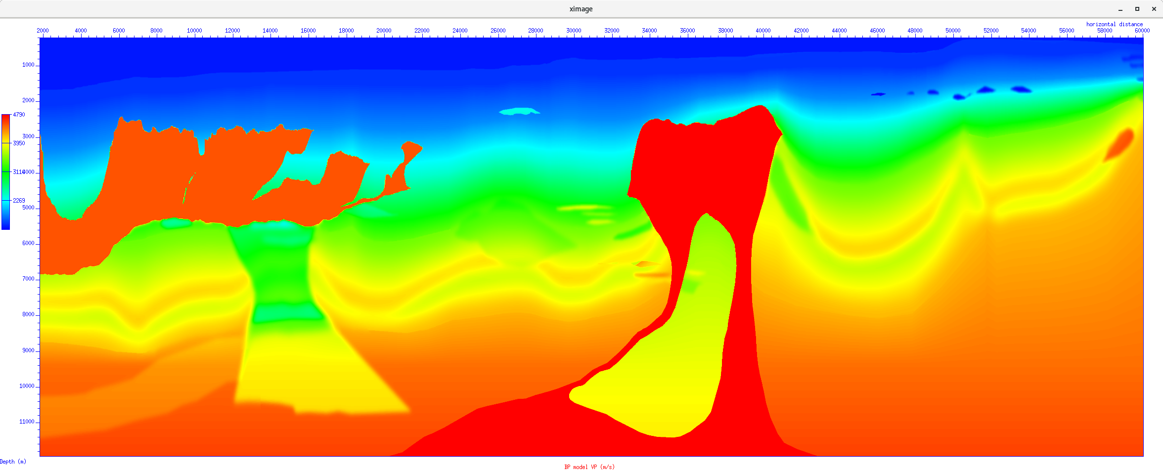
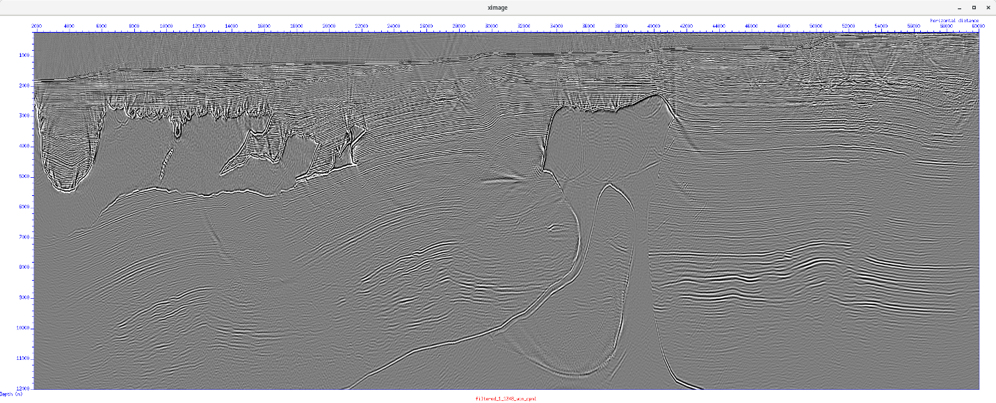
Figures 23 and 24 show the results of running the migration with the full data set using CPML and no boundary conditions.
For the results for CPML boundary conditions, as we did not remove multiples from the pre-stack data, those unwanted reflections are visible in the final image. The image looks pretty good as we have been using the correct velocity model. Laplace filter has been applied to filter the lower frequencies.
For the results with no boundary conditions, even if this picture looks similar to the Figure 24 , especially in the deeper part, we can see some non-realistic reflectors in the upper part.
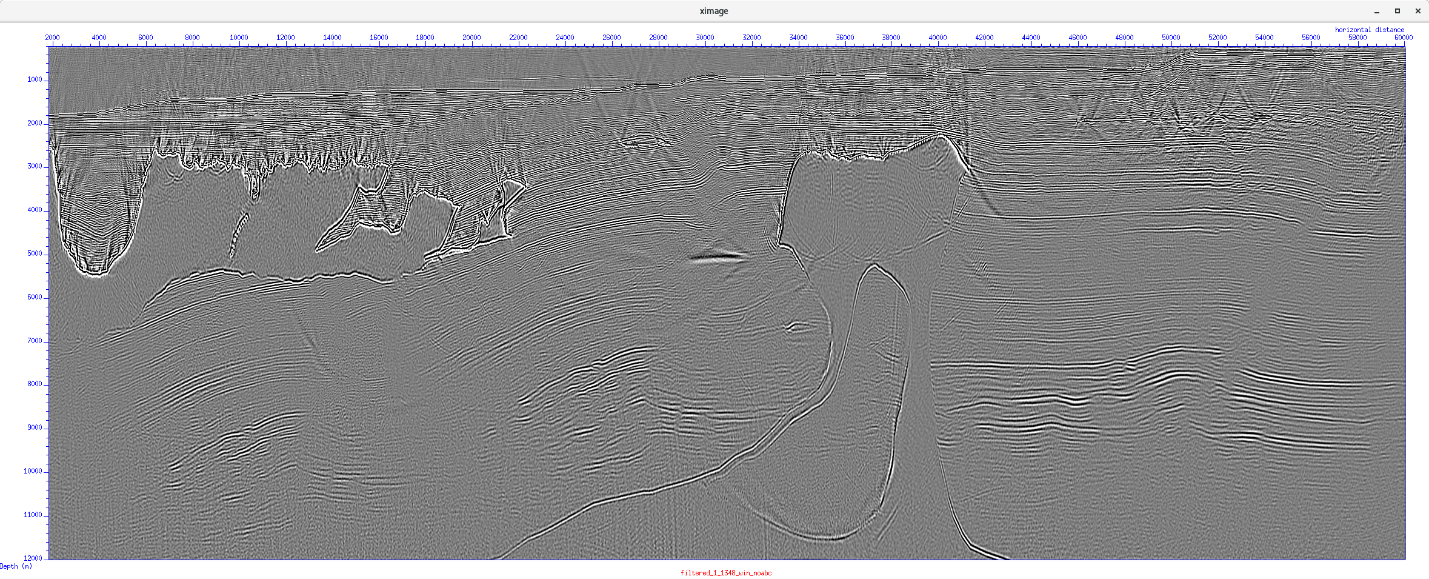
Figure 25 shows the relative amplitude of the waves in the model boundaries, showing the amount of attenuation over time produced by different types of boundary conditions and different number of grid points used in the boundaries.

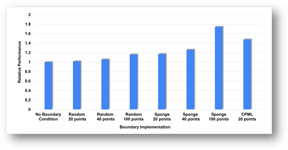
Figure 26 shows the computational performance of the different types of boundary conditions and number of grid points used in Figure 19. Review the trade-off between geophysical results (the amount of attenuation of the wavefront) and computational performance. For example, using a CPML boundary condition with 20 points is more computationally expensive than other options, but offers the best geophysical performance in terms of attenuation. A similar geophysical result can be obtained using a sponge boundary condition with 100 points, but at higher computational cost.
Summary
This tutorial explains how to profile and optimize a complex application using Intel Advisor. The example code used is RTM2D (Two-Dimensional Reverse-Time Migration), which is widely used in geophysical exploration to create images of the subsurface based on surface seismic data.
We run different types of analysis in Intel Advisor (Survey, Trip Counts and FLOP, Roofline, Dependencies) and compared Roofline chart results before and after optimizations to see the improvement.
Using RTM2D options, especially the boundary conditions and the snapshot management, we demonstrated how deep analysis can be performed through development choices, taking into account both the domain specific point of view (geophysics in this case) and the computational point of view (what is the fastest, what is the most efficient).
The best comparison here is between CPML with 20 boundary points, which is the most efficient to attenuate a wave but also expensive, and a sponge implementation, which can attenuate a wave only more points are added, and is even more expensive. We also point out the need for more geophysical comparisons using random velocity boundaries, especially in the areas of space sampling and propagated frequencies.
Apart from the standard vectorization guidance provided by Intel Advisor that gave us an example of false dependencies in the CPML and a nice speed-up, we also underlined the benefit of the Memory-level Roofline. Without digging deeply into the hardware counter collection, we can now quickly identify which memory level can be a performance bottleneck.
Resources
References
[1] Intel Corporation. 2020. Fact Sheet: oneAPI. (online)
[2] Intel Corporation. 2020. DPC++ overview. (online)
[3] Intel Corporation. 2020. Intel® Tiber™ AI Cloud
[4] Andreolli, C., Borges, L., Thierry, P. 2014. Eight Optimizations for 3-Dimensional Finite Difference (3DFD) Code with an Isotropic acoustic wave equation. (online)
[5] Metwaly, K., Elamrawi, K., Algizawy, E., Morad, K., Monir, I., ElBasyouni, M., Thierry, P. 2018. Accelerated Reverse Time Migration with optimized IO. ISC2018 Conference. (online)
[6] Imbert, D., Imadoueddine, K., Thierry, P., Chauris, H., Borges, L. 2011. Tips and tricks for finite difference and i/o‐less FWI. SEG, Expanded Abstracts, 30, 3174.
[7] Clapp, R. G. 2009. "Reverse time migration with random boundaries," SEG Technical Program Expanded Abstracts 2009, Society of Exploration Geophysicists, pp. 2809–2813.
[8] Lindstrom, P. 2014. Fixed-Rate Compressed Floating-Point Arrays. IEEE Transactions on Visualization and Computer Graphics, 20(12):2674-2683. (online)
[9] Intel Corporation. 2020. Intel® Integrated Performance Primitives Developer Reference. (online)
[10] Brightskies Inc. 2020. Brightskies RTM repository (Version 1.0.0). (online)
[11] Chattopadhyay, S and McMehan, G. 2008. Imaging conditions for prestack reverse-time migration. GEOPHYSICS 73: S81-S89.
[12] Billette, F. J., and S. Brandsberg-Dahl, 2005, The 2004 BP velocity benchmark: 67th Conference and Exhibition, EAGE, Extended Abstracts, B035.
[13] Berenger, J., 1994, A perfectly matched layer for the absorption of electromagnetic waves: Journal of Computational Physics, 114, 185–200.
[14] Cerjan, C., D. Kosloff, R. Kosloff, and M. Reshef, 1985, A nonreflecting boundary condition for discrete acoustic-wave and elastic-wave equations (short note): Geophysics, 50, 705–708
Notices and Disclaimers
Intel technologies may require enabled hardware, software or service activation.
No product or component can be absolutely secure.
Your costs and results may vary.
© Intel Corporation. Intel, the Intel logo, and other Intel marks are trademarks of Intel Corporation or its subsidiaries. Other names and brands may be claimed as the property of others.
No license (express or implied, by estoppel or otherwise) to any intellectual property rights is granted by this document.
The products described may contain design defects or errors known as errata which may cause the product to deviate from published specifications. Current characterized errata are available on request.
Intel disclaims all express and implied warranties, including without limitation, the implied warranties of merchantability, fitness for a particular purpose, and non-infringement, as well as any warranty arising from course of performance, course of dealing, or usage in trade.