We are excited to present our research on a nonmyopic approach to cost-constrained Bayesian optimization, which was recently published by the Conference on Uncertainty in Artificial Intelligence. This work was done in collaboration with scientists from Facebook and Amazon. In this summary, we’ll discuss the motivating factors behind this work.

The Default State of Hyperparameter Optimization: Measuring Progress by Iterations

Nearly all practical hyperparameter optimization packages attempt to determine optimal hyperparameters within a certain number of iterations. Let’s see how a user might run HyperOpt, Optuna, SKOpt, and SigOpt with a budget of 100 iterations:

Most optimizers have essentially the same interface: Plug in the objective you want to maximize/minimize and number of iterations you want to run. Most people take this interface for granted, but is it really the best way to optimize the objective? We argue that by asking for iteration count when we really care about something like cumulative training time, we are leaving performance on the table.

The Challenge: Varying Costs of Hyperparameter Evaluation

Measuring optimization progress by iterations is reasonable if each evaluation takes the same amount of time; however, this is often not the case in hyperparameter optimization (HPO). The training time

associated with one hyperparameter configuration may differ significantly from another. We confirm this in the study cited above, where we considered five of the most commonly used machine learning models:

• k-nearest neighbor (KNN)
• Multilayer perceptron (MLP)
• Support vector machine (SVM)
• Decision tree (DT)
• Random forest (RF)

Taken together, these models comprise the majority of general models that data scientists use. Note that deep learning models have been omitted, though our results hold for those as well.

We trained our five models on the commonly benchmarked OpenML w2a dataset using 5,000 randomly chosen hyperparameter configurations drawn from a standard search space. We then plotted a distribution of the resulting runtimes for each model (Figure 1). As you can see, the training times of each model vary greatly, often by an order of magnitude or more. This is because, for each model, a few

hyperparameters heavily influence not only model performance, but also training time (e.g., the layer sizes in a neural network or the number of trees in a forest). In fact, we have found that in nearly all practical applications, evaluation costs vary significantly in different regions of the search space.

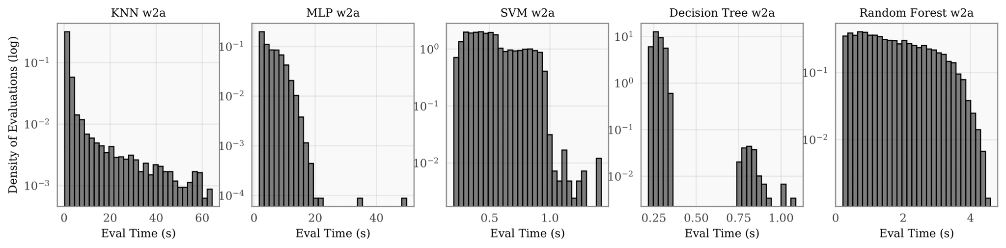
Figure 1. Runtime distribution, log-scaled, of 5,000 randomly selected points for the KNN, MLP, SVM, DT, and RF hyperparameter optimization problems. The x-axis of each histogram represents the runtime. The y-axis represents density (i.e., fraction of total evaluations).​

Consequently, the cumulative training time spent tuning these hyperparameters is not directly proportional to the number of iterations. In fact, it is entirely possible, according to the histogram above, for one optimizer to evaluate one hyperparameter configuration, for another optimizer to evaluate 100 points, and for both to take an equal amount of time doing so.

The Challenge: Handling a Heterogeneous Cost Landscape

We developed an optimizer that accounts for the varying cost landscape of the objective function and makes intelligent decisions about where to evaluate next. This is known as a cost-aware optimization routine. Instead of budgeting optimization by iteration count, our optimization routine takes into account an optimization budget measured by a cost metric, such as time. For example, instead of asking an optimization routine to compute the optimal hyperparameters in 100 iterations, we can instead ask it to compute the optimal hyperparameters in 100 minutes of training time. We might invoke such an optimization routine in the following way:

optimizer.minimize(func=objective, num_minutes=100)

This is an important research problem that the hyperparameter optimization community is actively prioritizing because, in practice, the user often has a cost budget that is expressed in money, time, or some other heterogeneous metric that constrains hyperparameter optimization.

On the Benefit of Being Cost-Aware

We developed a cost-aware optimization algorithm that we’ll call, “cost-aware Bayesian optimization (CA-BO).” To keep things simple, let’s consider an example comparing our CA-BO method to Optuna, a great open-source tool from Preferred Networks. Both optimizers are asked to maximize the binary classification accuracy of an XGBoost model in 100 optimization iterations. We see that as iteration continues, Optuna gradually outperforms CA-BO (Figure 2). The performance gap in this case is quite convincing. What might be happening? We would hope CA-BO at least performs as well as Optuna.

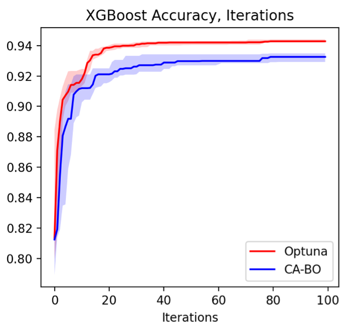
Figure 2. Comparison of CA-BO and Optuna for a fixed number of optimization iterations​

This gap exists because CA-BO is cost-aware. It recognizes that the evaluation cost varies and makes decisions accordingly. Let’s examine optimization performance when we account for varying evaluation cost, by replacing the x-axis with cumulative training time instead of iterations (Figure 3). We see that our CA-BO performs much better. Optuna eventually outperforms CA-BO, but only after CA-BO finishes running within its time budget (and it takes much longer to achieve comparable accuracy at nearly all times during optimization).

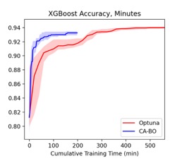
Figure 3. Comparison of CA-BO and Optuna based on training time

Side-by-side comparison highlights the stark difference between the cost-aware and cost-unaware optimization routines (Figure 4). On the right, we see that CA-BO finds superior hyperparameters within 200 minutes. On the left, we see that it finds worse hyperparameters within 100 iterations, which takes the cost-unaware approach more than 500 minutes to complete.

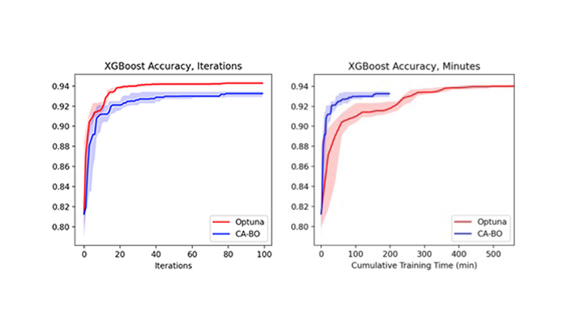
Figure 4. Side-by-side comparison of cost-aware and cost-unaware optimizer performance​

The picture on the left is the current state of HPO. The picture on the right is what developers trying to move models to production actually care about: a method that makes intelligent decisions based on the metric they care about.

Conclusions

CA-BO is a rapidly evolving class of algorithms for HPO. For more information about CA-BO, see our paper, which contains the technical details of our approach. For more information on other optimization techniques and applications, check out the SigOpt research page. Techniques like this are built into the SigOpt optimizer, one of the pillars of the SigOpt Intelligent Experimentation Platform. You can try out the optimizer and the rest of the platform for free by signing up today.

Related Content