Using the Monte Carlo method for simulating European options pricing
Goal
Compute nopt call and put European option prices based on nsamp independent samples.
Solution
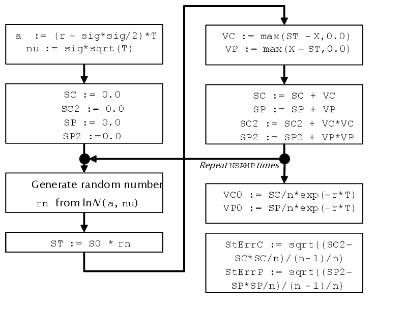
Use Monte Carlo simulation to compute European option pricing. The computation for a pair of call and put options can be described as:
Initialize.
Compute option prices in parallel.
Divide computation of call and put prices pair into blocks.
Perform block computation.
Deinitialize.
On OS X*, this solution requires oneMKL version 11.2 update 3 or higher.
Source code: see the mc folder in the samples archive available at https://software.intel.com/content/dam/develop/external/us/en/documents/mkl-cookbook-samples-120115.zip.
Initialize in OpenMP section
Create an OpenMP parallel section and initialize the MT2203 random number generator.
  #pragma omp parallel
    {
        ...
        VSLStreamStatePtr stream;

        j = omp_get_thread_num();

        /* Initialize RNG */
        vslNewStream( &stream, VSL_BRNG_MT2203 + j, SEED );
        ...
    }
This initialization model ensures independent random numbers streams in each thread.
Compute option prices in parallel
Distribute options across available threads.
  #pragma omp parallel
    {
        ...

        /* Price options */
      #pragma omp for
        for(i=0;i<nopt;i++)
        {
            MonteCarloEuroOptKernel( ... );
        }

        ...
    }
Divide computation of call and put prices pair into blocks
Divide generation of paths into blocks to maintain data locality for optimal performance.
    const int nbuf = 1024;
    nblocks = nsamp/nbuf;
    ...
    /* Blocked computations */
    for ( i = 0; i < nblocks; i++ )
    {
        /* Make sure that tail is correctly computed */
        int block_size = (i != nblocks-1)?(nbuf):(nsamp - (nblocks-1)*nbuf);
        ...
    }
Perform block computation
In the main computation, generate random numbers and perform reduction.
    /* Blocked computations */
    for ( i = 0; i < nblocks; i++ )
    {
        ...

        /* Generating block of random numbers */
        vdRngLognormal( VSL_RNG_METHOD_LOGNORMAL_ICDF, stream,
                        block_size, rn, a, nu, 0.0, 1.0 );

        /* Reduction */
      #pragma vector aligned
      #pragma simd
        for ( j=0; j<block_size; j++ )
        {
            st = s0*rn[j];
            vc = MAX( st-x, 0.0 );
            vp = MAX( x-st, 0.0 );
            sc += vc;
            sp += vp;
        }
    }

    *vcall = sc/nsamp * exp(-r*t);
    *vput  = sp/nsamp * exp(-r*t);
Deinitialize
Delete the RNG stream.
  #pragma omp parallel
    {
        ...
        VSLStreamStatePtr stream;
        ...
        /* Deinitialize RNG */
        vslDeleteStream( &stream );
    }
Routines Used
Task |
Routine |
|---|---|
Creates and initializes a random stream. |
vslNewStream |
Generates lognormally distributed random numbers. |
vdRngLogNormal |
Deletes a random stream. |
vslDeleteStream |
Discussion
Monte Carlo simulation is a widely used technique based on repeated random sampling to determine the properties of some model. The Monte Carlo simulation of European options pricing is a simple financial benchmark which can be used as a starting point for real-life Monte Carlo applications.
Let St represent the stock price at a given moment t that follows the stochastic process described by:
dSt = μStdt + σStdWt, S0
whereμ is the drift and σ is the volatility, which are assumed to be constants, W = (Wt)t≥ 0 is the Wiener process, dt is a time step, and S0 (the stock price at t = 0) does not depend on X.
By definition the expected value is E(St) = S0 exp(rt), where r is the risk-neutral rate. The previous definition of St gives E(St) = S0 exp((μ + σ2/2)t) , and combining them yields μ = r - σ2/2.
The value of a European option V(t, St) defined for 0 ≤t≤T depends on the price St of the underlying stock. The option is issued at t = 0 and exercised at a time t = T is called the maturity. For European call and put options the value of the option at maturity V(T, ST) is defined as:
Call option: V(T, ST) = max(ST - X, 0)
Put option: V(T, ST) = max(X - ST, 0)
where X is the strike price. The problem is to estimate V(0, S0).
The Monte Carlo approach to the solution of this problem is a simulation of n possible realizations of ST followed by averaging V(T, ST), and then discounting the average by factor exp(-rt) to get present value of option V(0, S0). From the first equation ST follows the log-normal distribution:
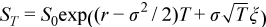
where ξ is a random variable of the standard normal distribution.
oneMKL provides a set of basic random number generators (BRNGs) which support different models for parallel computations such as using different parameter sets, block-splitting, and leapfrogging.
This example illustrates MT2203 BRNG which supports 6024 independent parameter sets. In the stream initialization function, a set is selected by adding j to the BRNG identifierVSL_BRNG_MT2203:
vslNewStream( &stream, VSL_BRNG_MT2203 + j, SEED );See Notes for Intel® MKL Vector Statistics for a list of the parallelization models supported by oneMKL VS BRNG implementations.
The choice of size for computational blocks, which is 1024 in this example, depends on the amount of memory accessed within a block and is typically chosen so that all the memory accessed within a block fits in the target processor cache.