Abstract
As with variable rate shading (VRS) Tier 1, the goal of VRS Tier 2 is to give developers additional control of where shading resources are used to produce an image. By reducing the shading rate in strategic areas, we can provide better performance, or use the saved time to spend more shading resources on pixels that will maximize the visual impact of what is seen on the screen. VRS Tier 2 gives developers more granularity than Tier 1 by making it possible to adjust shading rates per primitive, and/or by using a screen-space image. We explored this exciting new feature by implementing Velocity and Luminance Adaptive Rasterization (VALAR), which uses a combination of luminance and motion vectors to determine where the shading rate can be strategically reduced to increase performance without diminishing perceptible quality. Our work is derived from Lei Yang’s research on perceptually based shading metrics which also uses VRS6. In this paper, we explore the performance and quality trade-offs of our VALAR solution as a tool for game performance optimization.
Introduction
In this white paper, we discuss using VRS Tier 2 to improve performance in graphics applications, with a focus on Intel’s new discrete graphics products, Intel® ARC™. We first dive into an overview of VRS, explaining how it works, and review use-cases where VRS can attain performance gains with minimal impact on visual quality. We also discuss a sample project, released in tandem with this white paper—Implementing VRS Tier 2 within Microsoft*’s MiniEngine—which serves as a reference for those who are new to the technique or looking to add it to their game. The source code for the project will be available and linked to below.
We recommend the following white papers published if the reader is interested in more background information on VRS Tier 1:
- Getting Started With Variable Rate Shading Tier 1
- Variable Rate Shading Tier 1 Usage Guide With Unreal Engine
Variable Rate Shading
Variable rate shading is a technique for dynamically controlling rasterization, which gives developers more control of the trade-off between performance and visual quality. For example, if an object or region of the screen is undergoing motion blur, or objects are hidden behind smoke or fog, it often doesn’t make sense to spend much time shading when those results will be blurred before the user sees the final image. As display densities and resolutions have increased, each generation can double, or even quadruple, the number of pixels in the same region of space. This motivates the need for finer control of the amount of shading across the display to ensure we spend less time rendering low-visibility regions of an image, freeing up more time to render high-visibility regions of an image in higher quality.
![]()
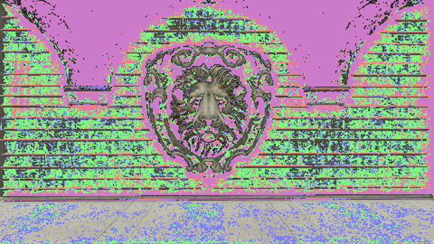
Figure 1. Visualization mode with the VRS shading rate overlaid onto the original image: You can see a drastic amount of pixels are being rendered at a different shading rate. Notice how a lot of the detail around the lion’s face is preserved at 1x1.

![]()
Figure 2. Zooming in on the previous image with focus on the lion’s head and mane, we can see the pixels where the shading rate has been reduced (left: control; middle: debug overlay; right: VRS Tier 2).
Variable-Rate Shading on Intel
Intel's ARC series gaming GPUs are Intel’s first line of GPUs that supports Microsoft DirectX 12* variable-rate shading at both Tier 1 and Tier 21. Previous generations of Intel graphics only supported VRS Tier 1, which we referred to as coarse pixel shading (CPS).
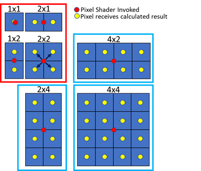
Figure 3. Coarse pixel sizes on Intel® hardware include the standard 1x1, 2x1, 1x2, and 2x2
As shown in Figure 3, Intel supports all the basic shading rates of 1x1, 2x1, 2x1 and 2x2 in the red box, and includes the extra shading rates of 2x4, 4x2, and 4x4 in the blue boxes. The red dot indicates where the pixel shader is invoked for a given size of coarse pixel. The yellow dots indicate where the invoked pixel shader calculated result will be propagated within the coarse pixel; see, for example, the 2x2 coarse pixel made of four fine pixels. The value is calculated at the midpoint of the 2x2 block of fine pixels, and that value is used for each of the four pixels that make the coarse pixel. The 1x1 pixel intentionally has a slight offset to show that both the invocation and the calculated result are at the same location.
These additional shading rates are important. They give the developer finer control over where rendering resources are focused. It is important to carefully consider where to apply these additional shading rates so as not to negatively impact the user experience. Finally, it is important to understand that while the shading rate is reduced, the depth, coverage, and stencil buffers are still calculated at full resolution. Edges that might be blurred by resolution scaling techniques, therefore, are preserved with VRS. This is shown in Figure 5.
VRS Use-Cases
Intel has been working with game developers to understand how to use these new shading rates and maintain visual quality. The ideal use-case for VRS is to leverage it in areas where the loss in quality and detail is imperceptible. Since VRS can reduce the number of pixel shader invocations, one use-case is draw calls that are pixel-shader-bound. Another use-case is when objects are moving quickly across the image plane and the loss of detail is unlikely to be perceived by the user. VRS also pairs nicely with objects when they are occluded by effects such as particles, fog, semi-transparent glass, or even depth-of-field effects. Reflections, particularly when blurred, are also potential candidates for the application of VRS.
Variable-Rate Shading in the Wild
The scenarios where reducing the shading rate while still maintaining the visual quality of the scene are similar for both VRS Tier 1 and Tier 2. The main upgrade from VRS Tier 1 is the additional degrees of control that VRS Tier 2 provides by allowing the shading rate to vary per-image-tile, and per-polygon.
At SIGGRAPH 2019, Intel presented several use-cases for variable-rate shading, including integration with depth-of-field, evaluating the impact of the speed of objects moving across the image plane, the visual impact of using VRS with atmospherics, and an initial integration into Epic’s Unreal Engine* [Lake, Strugar, Gawne et al. 2019]. At the Game Developers Conference (GDC) in 2020, Intel continued this applied research, and presented an integration of VRS Tier 1 into the Unreal Engine Material Editor, giving an artist complete control of shading rates for every material in a scene3. Using the per-material shading, Intel was able to demonstrate a range of use-cases, including VRS level of detail, VRS velocity with motion controls, and VRS volumes with particles.
The team of developers at The Coalition* successfully leveraged VRS Tier 1 and Tier 2 for performance gains in Gears 5 and Gears Tactics. The latter title achieved performance gains of up to 18.9% on a wide range of hardware, with minimal impact on visual quality; Gears 5 had gains of up to 14% with VRS Tier 24.
VRS Tier 1 with Depth of Field
One of our most promising new use-cases was the previously mentioned VRS integration with depth of field2. Using bounding boxes to approximate the scene geometry, the shading rate was adjusted for regions out of the main area of focus that would be blurred by the depth-of-field pass, then further tuned to handle cases of high specularity. This implementation of VRS was demonstrated to achieve a 16% performance improvement on the 3rd Gen Intel® Xeon® Scalable processor (formerly known as Ice Lake) at 2560x1600 resolution on the Amazon* Lumberyard Bistro dataset5.

Figure 4. Using Tier 1 variable-rate shading with depth of field to achieve a 16% performance saving with little to no loss in visual quality on the Amazon* Bistro scene
VRS Tier 1 in Chivalry II
Intel, along with publisher Tripwire*, presented the integration of VRS Tier 1 into Chivalry II3. We demonstrated that frame latency could be reduced with negligible loss in visual quality by adjusting the shading rate based on the camera direction and orientation. Resolution scaling is another means to achieve a reduction in shaded pixels independent of screen resolution. As a means of comparison, the presentation highlighted the improvements in edge preservation compared to a similar level of resolution scaling with a higher visual quality, as measured by the peak signal to noise ratio (PSNR). VRS was shown to provide the visual quality of an image that was scaled to 75% of the final displayed frame; yet the performance was as high as an image that was only the size of 50%-75% of the final frame in nine out of nine test scenes.

Figure 5. Image from Chivalry II showing the edge-preserving quality of variable-rate shading, compared to the same reduction in pixel shader invocations upscaled to the same display resolution
VRS Tier 2: Setting the Shading Rate and Shader Combiners
As mentioned earlier, Intel Arc Graphics will be the first Intel GPU to include support for VRS Tier 2. This adds the ability to set a shading rate via an image mask, set the shading rate per primitive, and combine all these shading rates together with a flexible shader-combiner API.
Setting a shading rate using an image mask
To use the image-based mask, where we set a per-tile shading rate, we create an image that is the size of the render target divided by a vendor-specific tile size. While other vendors may have coarser-grain tile sizes, Intel supports a fine-grained tile size of 8x8 pixels. For example, for a 1080p (1920x1080) render target we would create an 8-bit single channel image with a size of only 240x135 pixels. This image is used by the hardware at draw time to determine the shading rate to apply to each 8x8 region, before the pixel shaders are dispatched. This shading rate can be based on anything, but recent work has shown a contrast adaptive error metric6. to be useful, as well as Sobel edge-detector-based techniques7.
In addition to using this error metric, users could also lower the shading-rate of tiles completely covered by the UI, heads-up display (HUD), or other overlays, and combine these into a single image. Another use-case is foveated rendering, where the outer edges of the image are likely to be blurred. Lowering the shading rate is useful because the optics in a head-mounted display will be applying a significant distortion to the outermost pixels of the foveated region. In fact, this was one of the original motivations described in 2014 when Intel published an early paper on variable-rate shading8.

Figure 6. On Intel hardware, each pixel of the image mask represents an 8x8 tile of pixels on the render target.

Figure 7. Foveated shading-rate modes are a great way to save performance in cases such as virtual reality.
VRS shading rates can be set in a similar fashion as levels of detail (LOD) used in already existing game engines. By setting different far-and-near planes in the engine, the shading rate can decrease the farther away an object is from the camera. Using a VRS LOD system can work to reduce pixel shader invocations but if there are no atmospheric effects like fog, smoke, or particle effects, it is best not to be too aggressive with shading rates greater than 2x2.

![]()
Figure 8. Setting shading rates by specified LODs
The method that we have highlighted with our MiniEngine integration is what we call Velocity and Luminance Adaptive Rasterization (VALAR) which is an implementation of Nvidia*’s Adaptive Shading6. This method varies the shading rate using the previous frame’s color buffer, and, optionally, motion vectors. The current shading rate is based on the luminance of the tile, and optionally adjusted based on the motion vectors from the previous frame. The velocity buffer is used to reduce the shading rate while in motion, where the motion blur obscures any quality loss. This method uses a sensitivity threshold parameter to modify the aggressiveness of the shading rate. In our example, the sensitivity threshold can be set by the UI, or with a dynamic threshold that automatically selects the appropriate shading rate based on the current frame rate. The dynamic threshold uses a target FPS (Frames Per Second) to determine a threshold value between 0 and 1. For one example we used the following dynamic threshold:
Sensitivity Threshold = GPU Time / (1000 / FPS Target)

![]()
Figure 9. Velocity and luminance adaptive rasterization, with sensitivity threshold set to 0.15: You can see in this example how the dark archways and tapestry folds have a reduced shading rate.
Setting a shading rate per primitive
Setting the shading rate per primitive on the GPU is accomplished in a high-level shader language (HLSL) by setting a new shading rate on the provoking vertex, usually the first vertex of the polygon, with the HLSL Shader Model 6.4 system value SV_ShadingRate. There are a few instances where this could be used—for example, smoke particles start off small, and might suffer heavy overdraw. The screen-aligned smoke primitives can use a different shading rate depending on certain criteria—such as projected size or lifetime. Once the projected area reaches a certain size, or a certain amount of time has elapsed, the shading rate can be modified. Per primitive can also be used where per draw call might have been too coarse-grained—if a mesh might take up a significant part of the screen where portions of the object are going to be in fog, and other components out of fog. One example of this was discovered when we were rendering the Amazon Bistro. With VRS Tier 1, we had to hand-edit the geometry to chop it up into smaller segments. However, with VRS Tier 2 per primitive, we could have set a different shading rate for each polygon, based on what region the polygon lands in, in screen space, thus saving time for the artists that were forced to hand-tune the content to work with VRS Tier 1. While per tile is already proving a compelling VRS solution to game developers, we look forward to seeing how developers take advantage of being able to set the shading rate per polygon.
Shader Combiners: How to Combine Per-draw, Per-Image, and Per-Polygon Shading Rates
The additional flexibility of VRS Tier 2 introduces the following challenge: suppose I have set a shading rate per draw call, and I have set a different shading rate in the image mask for the destination pixels—who wins? With shading-rate combiners the answer is: whichever you want. Furthermore, you can also use the combiners to combine the values via addition, aggressively select the largest shading rate, or conservatively select the smallest. The combiners are merged by first evaluating the per-draw and per-polygon shading rates with the first shader combiner, and that result is sent to a second combiner to be combined with the per-image-tile shading rate. We can summarize this with the following:
ShadingRate = ShaderCombiner2(ShaderCombiner1 (per draw, per polygon), per tile).
The available shader combiners are addition (with a clamp to maximum-shading-rate supported), min, max, saturate, and passthrough. If no combiner is set, the default is passthrough. For additional details on the API refer to the Microsoft DirectX 12 documentation on VRS1.
Integration into the MiniEngine
The goal of this project was two-fold: this code sample can be used as a learning tool for others to add VRS Tier 2 into their own project, and we also wanted something that could be used for testing performance and quality on various hardware and settings. The MiniEngine UI exposes different shading-rate-related settings, per technique. We explore several different use-cases for VRS, some being realistic, and others contrived for the purpose of a sample. We will go deeper into these different techniques in later sections.
Source code links will be included at the end of the document. The project’s README will include build instructions, and list all the command-line options available.
Hardware Feature Queries
Before running any VRS-specific code, we must query the hardware to see if VRS is supported. If VRS is supported, we determine which variable rate shading tier is enabled. We also check if the additional shading rates (2x4, 4x2, and 4x4 respectively) are supported. Lastly, we query for the tile size that our hardware supports.
ID3D12Device* device;
D3D12_VARIABLE_SHADING_RATE_TIER ShadingRateTier = D3D12_VARIABLE_SHADING_RATE_TIER_NOT_SUPPORTED;
bool MeshShaderPerPrimitiveShadingRateSupported = false;
bool ShadingRateAdditionalShadingRatesSupported = false;
bool VariableRateShadingSumCombinerSuported = false;
UINT ShadingRateTileSize = 0;

// Initialize Device...

D3D12_FEATURE_DATA_D3D12_OPTIONS6 options6 = {};

// Get D3D12_OPTIONS6 Tier1 and Tier 2 support
if (SUCCEEDED(device->CheckFeatureSupport(
    D3D12_FEATURE_D3D12_OPTIONS6, &options6, sizeof(options6))))
{
     // Get Shading Rate Tier Supported
     ShadingRateTier = options6.Variable.ShadingRateTier;

     // Get VRS Tier 1 Additional Shading Rate Support
     if (ShadingRateTier >= D2D12_VARIABLE_SHADING_RATE_TIER_1
     {
         ShadingRateAddtiionalShadingRatesSupported =
        options6.AdditionalShadingRatesSupported;
     }

     // Get VRS Tier 2 Shading Rate Tile Size
     if (ShadingRateTier >= D2D12_VARIABLE_SHADING_RATE_TIER_2)
     {
         ShadingRateTileSize = options6.ShadingRateImageTileSize;
     }
}

D3D12_FEATURE_DATA_D3D12_OPTIONS10 options10 = {};

// Get D3D12_OPTIONS10 Additional Options
if (SUCCEEDED(device->CheckFeatureSupport(
    D3D12_FEATURE_D3D12_OPTIONS10, &options10, sizeof(options10))))
{
     // Get Shading Rate Sum Combiner Support
     VariableRateShadingSumCombinerSupported =
    options10.VariableRateShadingSumCombinerSuppoered;

     // Get Shading Rate Per Primitive Report
     MeshShaderPerPrimitiveShadingRateSupported =
    options10.MeshShaderPerPrimitiveShadingRateSupported;
}

// Use/Store VRS Tier 1 & Tier 2 Settings...
Figure 10. Code sample showing how to query a device for VRS hardware support and feature levels.
VRS Tier 1
Using VRS Tier 1 is straightforward. Before we draw, we simply set the default per-pass shading rate using RSSetShadingRate. Note that nullptr is passed in for the shading rate combiners, as these can only be used with Tier 2.
// Make Sure Shading Rate Tier 1 is Supported
if (VRS::ShadingRateTier == D3D12_VARIABLE_SHADING_RATE_TIER_1)
{
     // Set a Default “Per-Pass” Shading Rate, Optionally Use a Configurable Variable
    gfxContext.GetCommandList()->RSSetShadingRate(D3D12_SHADING_RATE_1X1, nullptr);
}
Figure 11. Example of how to set VRS Tier 1 shading rate
VRS Tier 2
Setting the shading rate with Tier 2 using the DirectX 12 API is straightforward. First, we set the per-pass shading rate as we do with Tier 1. This time, however, we need to pass in the shading-rate combiners, instead of nullptr. We transition the VRS Tier 2 buffer to a shading-rate source state, then set the shading-rate buffer using RSSetShadingRateImage. Note that the size of our VRS Tier 2 buffer is only one-eighth of the size of our color buffer; this is because each pixel of our image mask corresponds to the shading-rate tile size supported by the hardware.
//Make Sure VRS Tier 2 is Supported
if (VRS::ShadingRateTier == D3D12_VARIABLE_SHADING_RATE_TIER_2)
{
     // Setup Shading Rate Combiners
     D3D12_SHADING_RATE_COMBINER shadingRateCombiners[2] = {
              D3D12_SHADING_RATE_COMBINER_PASSTHROUGH  ,
              D3D12_SHADING_RATE_COMBINER_OVERRIDE
     };

     // Set the Default “Per-Pass” Shading Rate, and Shading Rate Combiners
     gfxContext.GetCommandList()->RSSetShadingRate(
        D3D12_SHADING_RATE_1X1, shadingRateCombiners);

     // Transition VRS Tier 2 buffer to D3D12_RESOURCE_STATE_SHADING_RATE_SOURCE
     gfxContext.TransitionResource(g_VRSTier2Buffer,
        D3D12_RESOURCE_STATE_SHADING_RATE_SOURCE, true);

     // Set Shading Rate Buffer using RSSetShadingRateImage
     gfxContext.GetCommandList()->RSSetShadingRateImage(
        g_VRSTier2Buffer.GetResource());
}
Figure 12. This code snippet shows us grabbing the shading-rate combiners that were set in the debug UI to then use them to set the shading rate. We also make sure to set our shading-rate image to our image mask.
You will want to control the scope of your VRS Tier 2 shading-rate image commands. Using VRS Tier 2 in some passes may introduce unexpected visual corruption if you are applying a shading rate image to the full scope of your command list. To disable VRS Tier 2 for a given command list you can call RSSetShadingRateImage with a value of nullptr instead of a shading-rate buffer.
Velocity and Luminance Adaptive Rasterization (VALAR)
The VALAR algorithm uses a single compute shader with three unordered-access views (UAVs) and nine constant buffer values. The UAV buffers passed into the compute shader are: the VRS Tier 2 shading-rate buffer, the main render-target color buffer, and an optional velocity buffer. The constant buffer values passed are the render-target width/height, the shading-rate tile size returned by the D3D12_FEATURE_D3D12_OPTIONS6 struct, and several values and options used to parameterize the VALAR algorithm:
Sensitivity Threshold: The threshold for determining the Just Noticeable Difference—common values to test are 0.25 (Quality), 0.5 (Balanced), and 0.75 (Performance)
Env. Luma: Global illumination additively increases the overall luminance in the Just Noticeable Difference threshold equation.
K: This is the quarter-rate shading modifier, which increases the aggressiveness of the 4x4, 4x2, and 2x4 shading-rates. Lower values will result in higher-quality images.
Use Motion Vectors: Includes motion vectors in the Sensitivity Threshold comparisons which will adjust the mean-squared error based on tile minimum velocity; there is a marginal performance cost for the additional velocity-math and velocity-fetches in the compute shader when using this feature.
Use Weber-Fechner (Luminance Differences): The default algorithm is a luminance approximation, but we can use a more precise algorithm based on Weber’s Contrast Law using neighboring pixel luminance values. There is a time cost, but it comes with higher quality and precision. Test it in areas of high-frequency content, or when the sensitivity threshold is greater than 0.5, or 0.75.
Weber-Fechner Constant: Scales the luminance differences when using Weber’s Contrast Law for Brightness Sensitivity.
// Create Descriptor Handle Array for UAVs
D3D12_CPU_DESCRIPTOR_HANDLE Pass1UAVs[] =
{
    g_VRSTier2Buffer.GetUAV(),
    g_SceneColorBuffer.GetUAV(),
    g_VelocityBuffer.GetUAV()
};

// Set Root Signature with 3 UAVs & 9 Constant Buffer Values
Context.SetRootSignature(ContrastAdaptiveRootSig);

// Set Constant Buffer Values
Context.SetConstant(0, 0, (UINT)g_SceneColorBuffer.GetWidth());
Context.SetConstant(0, 1, (UINT)g_SceneColorBuffer.GetHeight());
Context.SetConstant(0, 2, (UINT)ShadingRateTileSize);
Context.SetConstant(0, 3, (float)ContrastAdaptiveSenstivityThreshold);
Context.SetConstant(0, 4, (float)ContrastAdaptiveK);
Context.SetConstant(0, 5, (float)ContrastAdaptiveWeberFechnerConstant);
Context.SetConstant(0, 6, (float)ContrastAdaptiveWeberFechnerConstant);
Context.SetConstant(0, 7, (bool)ContrastAdaptiveUseWeberFechner);
Context.SetConstant(0, 8, (bool)ContrastAdaptiveUseMotionVectors);

// Set UAV Dynamic Descriptors in Compute Shader
Context.SetDynamicDescriptors(1, 0, _countof(Pass1UAVs), Pass1UAVs);

// Transition UAV Resources to UNORDERED_ACCESS State.
Context.TransitionResource(g_VRSTier2Buffer,
     D2D12_Resource_State_UNORDERED_ACCESS);
Context.TransitionResoruce(g_Scene(ColorBuffer,
     D3D12_Resource_State_UNORDERED_ACCESS);
Context.TransitionResource(g_VelocityBuffer,
     D3D12_Resource_State_UNORDERED_ACCESS);

// Set Pipeline State Object
Context.SetPipelineState(VRSContrastAdaptiveCS);

// Dispatch 1/8th Target Width by 1/8th Target Height Threads for 8x8 Tile Size
// Dispatch 1/16th Target Width by 1/16th Target Height Threads for 16x16 Tile Size
Context.Dispatch((UINT)ceil((float)g_SceneColorBuffer.GetWidth() / (float)ShadingRateTileSize);
                 (UINT)ceil((float)g_SceneColorBuffer.GetHeight() / (float)ShadingRateTileSize)),
Figure 13. Setting up our compute shader
After setting the uAVs and constant-buffer values, a thread group with Target.Width() / ShadingRateTileSize by Target.Height() / ShadingRateTileSize dimensions is dispatched. For example, a 1080p render target running on Intel hardware would dispatch 1920/8 x 1080/8 thread groups for a total of 375 thread groups. For a shader executing on Intel, the number of threads per thread group would be equal to [numthreads(8, 8, 1)], and if the tile size was 16x16, the number of threads would be [numthreads(16, 16, 1)], to get the correct mapping for the VRS Tier 2 buffer.
VALAR Implementation

Figure 14. Simplified shader phases diagram
Broadly, the VALAR compute shader is composed of two main phases: First, the parallelized luminance differencing and (optional) velocity computation used to pre-compute the luminance and velocity for a given tile. Second, a serialized phase that computes the luminance mean-squared error (MSE) and Just Noticeable Difference (JND) evaluation using the sensitivity threshold to select the proper shading rate for the tile. In our implementation, we include three different implementations:
- An unoptimized base implementation so we can quantify speedup.
- An implementation that relies on wave intrinsics, and some additional group shared memory.
- And, an optimization where we leveraged atomics and wave intrinsics together.
Our optimized implementations provide close to a 4x speedup over the unoptimized implementation.
VALAR Parallel Luminance Differencing, and Minimum Tile Velocity
In the first phase of the compute shader, luminance and velocity values are fetched from their associated buffers using the Dispatch Thread ID to determine the correct UV location.

Figure 15. Parallelized compute-shader phase one block flowchart
After fetching the RGB color value for a given pixel, it is linearized, and then converted to the luminance scale, using the following conversion: dot(LinearRGB, float3(0.212671, 0.715160, 0.072169)).
// Use Dispatch Thread ID to Determine UV of the color buffer UAV
const uint2 PixelCoord = DTid.xy;

// Fetch Colors from Color Buffer UAV
const float 3 color          = FetchColor(PixelCoord);
const float 3 colorXMinusOne = FetchColor(uint2(PixelCoord.x - 1, PixelCoord.y));
const float 3 colorYMinusOne = FetchColor(uint2(PixelCoord.x, PixelCoord.y - 1));

// Convert RGB to luminance values
const float pixelLuma          = RGBToLuminance(color * color);
const float pixelLumaXMinusOne = RGBToLuminance(colorXMinusOne * colorXMinusOne);
const float pixelLumaYMinusOne = RGBToLuminance(colorXMinusOne * colorYMinusOne);
Figure 16. Fetching RGB and converting linearized RGB to luminance
After converting the color-buffer RGB float3 value into a scalar luminance float value, the compute shader computes the difference between neighboring luminance contrast, on both the x and y axis. We used two methods to decide the local contrast. There is a simplified approximation mode, and a more precise “Weber-Fechner” mode based on Weber-Fechner's law6.
if (UseWeberFechner)
{
     // Use Weber Fechner to create brightness sensitivity divisor.
     float minNeighborLuma = ComputeMinNeighborLuminance(GTid.xy);
     float BRIGHTNESS_SENSITIVITY = WeberFechnerConstant * (1.0 - saturate(minNeighborLuma * 50.0 - 2.5));

     // When using Weber-Fechner Law https://en.wikipedia.org/wiki/Weber%E2%80%93Fechner_law
     localWaveLumaSumX = WaveActionSum(abs(pixelLuma - pixelLumaXMinusOne) /
                                                (min(pixelLuma, pixelLumaXMinusOne) + BRIGHTNESS_SENSITIVITY));

     // When using Weber-Fechner Law https://en.wikipedia.org/wiki/Weber%E2%80%93Fechner_law
     localWaveLumaSumX = WaveActionSum(abs(pixelLuma - pixelLumaXMinusOne) /
                                                (min(pixelLuma, pixelLumaXMinusOne) + BRIGHTNESS_SENSITIVITY));
     // When using Weber-Fechner Law https://en.wikipedia.org/wiki/Weber%E2%80%93Fechner_law
     localWaveLumaSumX = WaveActionSum(abs(pixelLuma - pixelLumaXMinusOne) /
                                                (min(pixelLuma, pixelLumaXMinusOne) + BRIGHTNESS_SENSITIVITY));
}
else
{
     //Satisfying Equation 2. http://leiy.cc/publications/nas/nas-pacmcgit.pdf
     localWaveLumaSumX = WaveActiveSum(abs(pixelLuma - pixelLumaXMinusOne) / 2.0);

     //Satisfying Equation 2. http://leiy.cc/publications/nas/nas-pacmcgit.pdf
     localWaveLumaSumY = WaveActiveSum(abs(pixelLuma - pixelLumaYMinusOne) / 2.0);
}
Figure 17. Computing local contrast with Weber’s Contrast Law, and approximate contrast
Weber-Fechner Luminance Differences
To compute a more precise luminance difference using Weber’s Contrast Law, the VALAR algorithm computes the minimum luminance of a 3x3 grid with the current pixel at the center. The minimum luminance is then converted into a brightness sensitivity range and scaled using the WeberFechnerConstant constant-buffer value6.
float BRIGHTNESS_SENSITIVITY = WeberFechnerConstant * (1.0 - saturate(minNeighborLuma * 50.0 - 2.5));
After the brightness sensitivity is computed Weber’s Contrast Law is used to compute the contrast in both the x and y axis:
abs(pixelLuma - pixelLumaXMinusOne) / (min(pixelLuma, pixelLumaXMinusOne) + BRIGHTNESS_SENSITIVITY
abs(pixelLuma - pixelLumaXMinusOne) / (min(pixelLuma, pixelLumaXMinusOne) + BRIGHTNESS_SENSITIVITY
Approximate Luminance Differences
Weber’s Contrast Law can be simplified with an approximation which results in improved performance but slightly lower quality. Instead of using brightness sensitivity, it is replaced by a constant value of 2.0 as follows:
abs(pixelLuma - pixelLumaXMinusOne) / 2.0;
abs(pixelLuma - pixelLumaYMinusOne) / 2.0;

Figure 18. Color buffer converted to luminance
Next, the shader will optionally compute the minimum wave-lane velocity using WaveActiveMin(). Note, when using wave intrinsics, it is best to query the device for WaveOps Support (e.g., D3D12_FEATURE_DATA_D3D12_OPTIONS1::WaveOps). The MiniEngine stores motion vectors in a packed format, which need to be unpacked when sampling the underlying motion-vector UAV, prior to conversion to the magnitude of the vector using the length() function.
// Sample & Unpack Velocity Data from Velocity Buffer
const float3 velocity = UnpackVelocity(VelocityBuffer[PixelCoord]);
// Get the magnitude of the vector and determine minimum value in wave lane
localWaveVelocityMin = WaveActiveMin(length(velocity));
Figure 19. Using WaveActiveMin to find the minimum velocity per-wave
At this point, GroupMemoryBarrierWithGroupSync() is called to allow all threads to compute their per-pixel luminance and velocity values, before moving to the serialized portion of the shader.
VALAR Serialized Error Estimation and Just Noticeable Difference Threshold
Once all the threads in the parallel phase have synchronized, the luminance values are averaged together. This is done for the entire tile as well as the luminance differences for the x and y axis.

Figure 20. Phase two average luminance, JND thresholding, and mean-squared error flowchart
The original image is essentially converted into one-eighth or one-sixteenth the size of the original luminance image, depending on ShadingRateTileSize, defined by the hardware vendor. The WaveActiveSum partial sums from the parallelized phase are stored in wave-lane bins in a groupshared memory array (e.g. groupshared float waveLumaSum[64]), and are then summed and averaged together.
// Loop through waveline sized bins to sum partial sums
for (int i = 0; i < (NUM_THREADS / waveLaneCount); i++
{
     totalTileLuma += saveLumaSum[i];
     totalTileLumaX += waveLumaSumX[i];
     totalTileLumaY += waveLumaSumY[i];
     minTileVelocity = min(minTileVelocity, saveVelocityMin[i];
}

// Compute Average Luminance of Current Tile
const float avgTileLuma = totalTileLuma / (float)NUM_THREADS;
const float avgTileLumaX = totalTileLumaX / (float)NUM_THREADS;
const float avgTileLumaY = totalTileLUmaY / (float)NUM_THREADS;
Figure 21. Summing WaveActiveSum partial sums and averaging luminance values
Now that the average tile luminance has been computed, the JND threshold can be calculated by adding the Environmental Luma constant-buffer value to the average tile luminance, and then scale by the sensitivity threshold constant-buffer value.
// Satisfying Equation 15. http://leiy.cc/publications/nas/nas-pacmcgit.pdf
const float jnd_threshold = SensitivityThreshold * (avgTileLuma + EnvLuma);
Figure 22. Computing a just noticeable difference threshold
Once the JND threshold is determined, the mean square error (MSE) value is computed for each of the X & Y luminance differences in the tile using the sqrt() function.
// Compute the MSE error for Luma >/Y derivatives
const float avgErrorX = sqrt(avgTileLumaX);
const float avgErrorY = sqrt(avgTileLumaY);
Figure 23. Computing MSE for X and Y luma differences

Figure 24. (Optional) Velocity scaling, JND thresholding, and per-axis shading-rate combiners
Before performing the JND threshold test, the minimum tile velocity can be combined with the K constant buffer value to scale the jnd_threshold value proportionally to the minimum velocity in the tile. The closed-form equations that are used to modify the MSE values are as follows:
// Satisfying Equation 20. http://leiy.cc/publications/nas/nas-pacmcgit.pdf
velocityHError = pow(1.0 / (1.0 + pow(1.05 * minTileVelocity, 3.10)), 0.35);
// Satisfying Equation 21. http://leiy.cc/publications/nas/nas-pacmcgit.pdf
velocityQError = K * pow(1.0 / (1.0 + pow(0.55 * minTileVelocity, 2.41)), 0.49);
Figure 25. Compute half-rate and quarter-rate velocity modifiers
Determining the full-rate, half-rate, or quarter-rate shading for a given tile is a simple if-else statement that also scales the per-axis luminance MSE value by the (optional) velocity error metric. First, the half-rate velocity approximation is used to scale the MSE value, and if it is greater than or equal to the jnd_threshold value, a full-rate shading rate (1X) is selected. If the full-rate shading test fails, the quarter-rate shading test is performed by scaling the MSE value by the quarter-rate velocity error metric. If it is less than the jnd_threshold value, quarter-rate shading rate (4X) is selected, otherwise it will default to half-rate shading (2X).
// Satisfying Equation 16. For X
// http://leiy.cc/publications/nas/nas-pacmcgit.pdf
if ((velocityHError * avgErrorX) >= jnd_threshold)
{
    xRate = D3D12_AXIS_SHADING_RATE_1X;
}
// Satisfying Equation 14. For Quarter Rate Shading for X
// http://leiy.cc/publications/nas/nas-pacmcgit.pdf
else if ((velocityQError * avgErrorX) < jnd_threshold)
{
    xRate = D3D12_AXIS_SHADING_RATE_4X;
}
// Otherwise Set Half Rate Shading Rate
else
{
    xRate = D3D12_AXIS_SHADING_RATE_2X;
}
Figure 26. Example of per-axis (x-axis) JND threshold-test
When the motion vectors from the previous frame are disabled, the half-rate velocity error metric is set to 1.0, and the quarter-rate velocity error metric will be equal to the K value in the constant buffer. The JND threshold test is done on a per-axis basis, which will result in D3D12_AXIS_SHADING_RATE value for both the x and y axis.

Figure 27. Converting average tile-luminance to per-axis shading-rates, using the JND threshold algorithm
The per-axis shading rates are then combined to create a D3D12_SHADING_RATE value, using the D3D12_MAKE_COURSE_SHADING_RATE macro provided by Microsoft in the DirectX 12 API.
#define D3D12_MAKE_COARSE_SHADING_RATE(x,y) ((x) << D3D12_SHADING_RATE_X_AXIS_SHIFT | (y))

Figure 28. Per-axis shading rates combined to produce the final shading-rate buffer
Finally, the Group ID of the serialized thread is used to write the combined D3D12_SHADING_RATE value to the VRS Tier 2 buffer, at which point the shader execution completes.
SetShadingRate(Gid.xy, D3D12_MAKE_COARSE_SHADING_RATE(xRate, yRate));
The final VRS buffer is then used as a shading-rate image for the next frame. There are minimal changes needed to enable VALAR in a rendering pipeline which simply applies the VRS Buffer with RSSetShadingRateImage(), prior to rendering the color buffer.
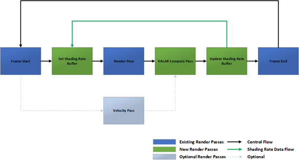
Figure 29. VALAR-enabled rendering pipeline
We show a significant reduction in pixel-shader invocations which scale proportionally with the sensitivity threshold using VALAR in Microsoft’s DX12 MiniEngine rendering pipeline. In some scenes, there was up to a 1.88x reduction in pixel-shader invocations when the sensitivity threshold was set to Performance (t = 0.75) and rendered at 4K resolution. Quality and Balanced modes had smaller reductions in pixel-shader invocations but were still consistent with the sensitivity threshold value selected.

Figure 30. Pixel-shader reductions for quality (t=0.25), balanced (t=0.50), and performance (t=0.75) modes in the MiniEngine (*Pre-production hardware, figures subject to change)
The overall reduction in pixel-shader invocations may result in performance gains of up to 1.12x on a 4K (3840x2160) render target in some scenes.

Figure 31. Content-dependent speedups with Microsoft’s MiniEngine using VALAR. (*Pre-production hardware, figures subject to change)
The gains seen when using VALAR in the MiniEngine are content-dependent and may vary based on the amount of content in a game as well as the performance of the target GPU.
Visual Results and Performance
We can now look at the quality differences between different sensitivity threshold settings of VALAR. For our experiments, we chose three sensitivity thresholds that we will refer to as Quality (t = 0.25), Balanced (t = 0.50), and Performance (t = 0.75). As mentioned previously, when using a Just Noticeable Difference algorithm to set the appropriate shading rates, the loss in quality may not be visually perceptible to the user.
However, how something looks can often be subjective, and we would like to measure the differences in quality with a more scientific approach. To do this, we can use image-quality assessment metrics, such as the Mean-Squared Error (MSE), Peak Signal to Noise Ratio (PSNR), Structured Similarity Indexing Method (SSIM), or Feature Similarity Indexing Method (FSIM)9. While each of these metrics are different from one another, they all work the same, in that they compare an original reference image to a test image.
To collect the quality metrics for analysis, three main tools were used: Image Magick*10. for PSNR and image diffs, Nvidia ꟻLIP*11, for Mean Error and heatmapped diffs, and Nvidia ICAT,*12. for image comparison. To make the tests reproducible, we move the camera to predefined positions within the scene and use a readback buffer paired with stb_image to capture the screenshot13. Three different areas in the Crytek* Sponza scene were analyzed: a broad first-floor view; a close-up of one of the tapestries; and a focus on one of the lion-head statues. For each of these camera positions, three different sensitivity thresholds were compared to the control image.

![]()
Figure 32. Even though there are quality differences between the control and VRS image, Nvidia ꟻLIP* doesn't detect a perceptible difference.
Metric Differences
The metrics used to analyze quality tell us different things. PSNR measures quality logarithmically in decibels, whereas ꟻLIP approximates perceptual difference as an accumulated error using a variety of metrics. We primarily used the mean error metric to estimate visual quality loss. PSNR can detect noise and show objective differences between two images; however, these variances may not be visually noticeable. It is common for image-detail comparisons to use a generic calculation to determine differences between images. This will treat all color channels similarly. The human eye, however, perceives gradual changes between red, green, and blue differently, with each having varying levels of noticeable significance. By taking this aspect into account, we believe ꟻLIP is a better representation of human perception. The two bar-charts below show this by comparing the same images. You can also see this in the image above. There are areas of the image with their shading-rate reduced, yet the ꟻLIP output tells us these are not perceptible differences in those regions.
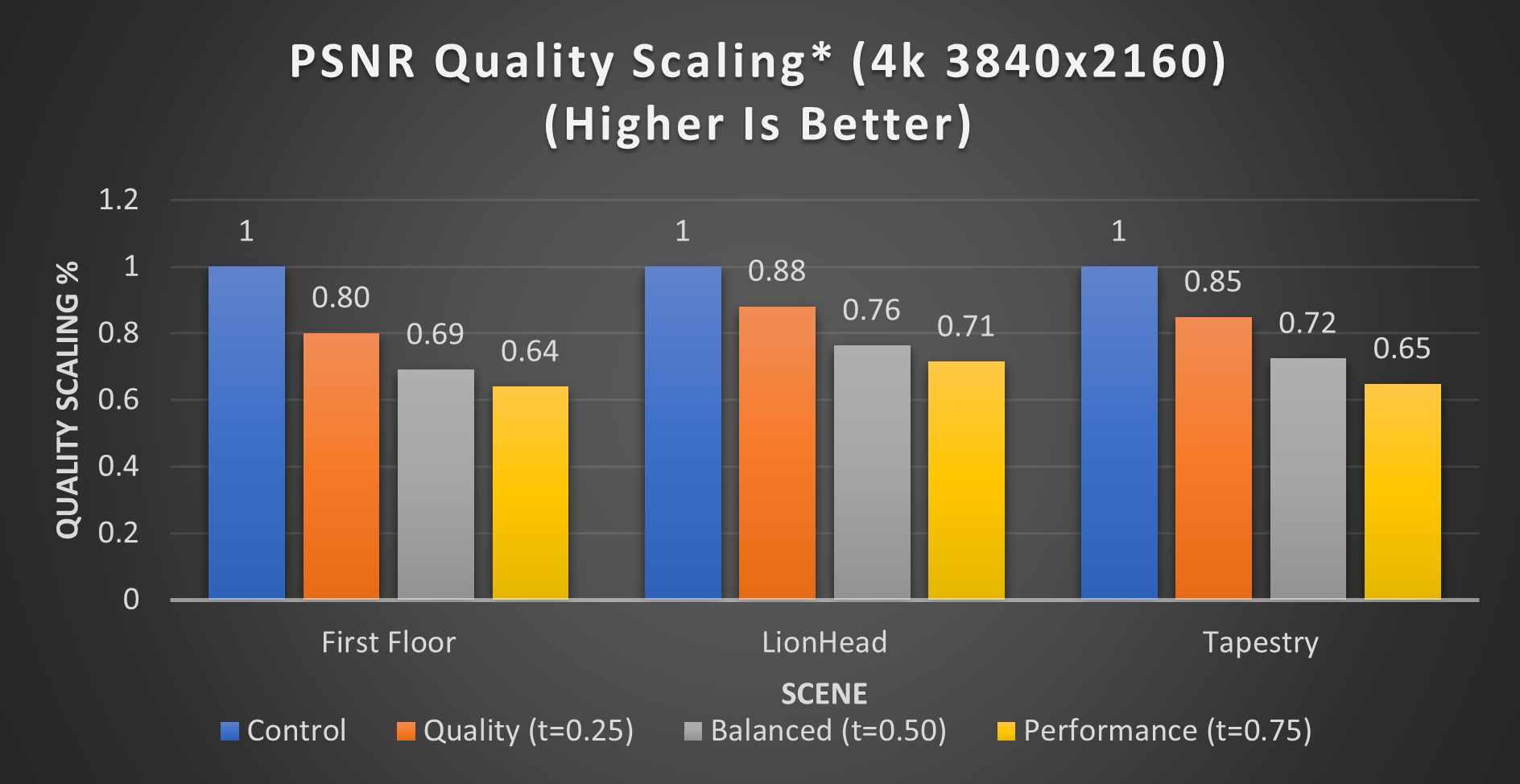
Figure 33. PSNR quality tradeoff scaling (4k 3840x2160) (*Pre-production hardware, figures subject to change)
As expected, the more aggressive the shading rate, the lower the quality. When comparing the two quality metrics, we can infer that there are significant portions of the image that are different, yet not discernible to the naked eye.
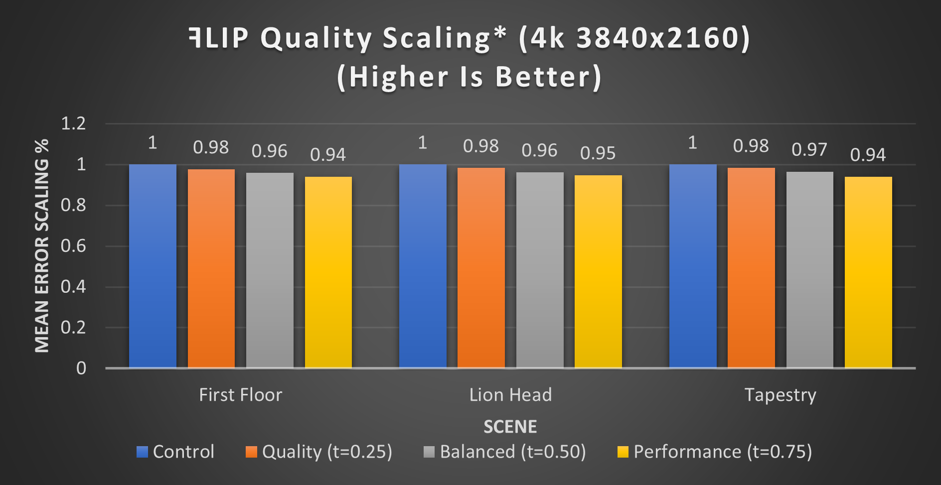
Figure 34. ꟻLIP mean error scaling (4k 3840x2160) (*Pre-production hardware, figures subject to change)
Approximate versus Weber-Fechner Luminance: Performance
As discussed previously, we investigated two different modes to determine luma differences, and described how each one is implemented. But what are the performance differences? It comes as no surprise that, on average, the Approximate Luma Difference algorithm results in more speedup than the Weber-Fechner method, due to the additional neighbor fetches of the Weber-Fechner method. For example, using the performance setting in our tapestry scene, Approximate Luma produced a scaled speedup of 1.11x, whereas the Weber-Fechner algorithm produced a 1.07x speedup. That is not the full story, however, as the Weber-Fechner cost is incurred in the hopes it improves the visual quality.

Figure 35. Approximate Luma differences algorithm performance scaling (4K 3840x2160) (*Pre-production hardware, figures subject to change)

Figure 36. Weber-Fechner Luma differences algorithm performance scaling (4k 3840x2160) (*Pre-production hardware, figures subject to change)
Approximate versus Weber-Fechner Luminance: Quality
If Approximate Luma is more performant, then why would you use Weber-Fechner? We can observe that, in some cases, Weber-Fechner provides better quality at a given level of performance. Weber-Fechner specifically seems to thrive when the sensitivity threshold is above 0.5, otherwise it struggles to compete with Approximate Luma. Determining when to use Weber-Fechner is scene-dependent, but the general heuristic is that Weber-Fechner can be beneficial in scenes with high-frequency content.

Figure 37. Approximate Luma ꟻLIP quality scaling (4k 3840x2160) (*Pre-production hardware, figures subject to change)

Figure 38. Weber-Fechner Luma ꟻLIP quality scaling (4K 3840x2160) (*Pre-production hardware, figures subject to change)
ꟻLIP was used to generate a series of histograms that we used to compare image quality for Quality, Balanced, and Performance modes, using both Approximate Luma Differencing and Weber-Fechner Luma Differencing. As you can see in the figure below, the number of pixels with the lower ꟻLIP error-rate are largely concentrated toward the 0.0 error-rate on the left-hand side of the histogram. This is reinforced simply by examining the third weighted-quartiles for each histogram. This helps indicate that the images generated using the Weber-Fechner Luma differences method, with VRS, have a more perceptually similar image to the original, compared to the images generated using the approximate Luma differences method. In effect, by utilizing Weber-Fechner's contrast law, we are allowing VRS to optimally target more visually significant portions of the image with higher shading-rates, while deprioritizing areas with less visible differences.

Figure 39. Comparing these histograms highlight that Weber-Fechner accumulates less error, while the Approximate algorithm isn’t as accurate. We can also see that the largest difference between the two methods was in performance mode. (*Pre-production hardware, figures subject to change)
We can also inspect the differences between the two methods visually. In the image below, notice how Weber-Fechner is less aggressive than the Approximate method. The brick wall utilizes a lower shading rate, and a large portion of the floor has its quality maintained at 1x1. However, in other areas, such as the archway, both perform somewhat similarly.

![]()
Figure 40. Left, Approximate medium; Right, Weber-Fechner medium
In summary, there are trade-offs between the Approximate Luma method and Weber-Fechner. Both retain quality in important areas of the scene. Approximate Luma is more performant, but sacrifices quality. Weber-Fechner can achieve higher fidelity, albeit with a performance cost. It is up to the developer to choose what suits their needs best, and which is a better fit for their game.
Summary
We believe that VRS should be integrated as a first-class feature of any DirectX 12 Ultimate rendering pipeline. The API, when combining per-draw, per-tile, and per-primitive support, provides a rich palette for developers to explore solutions that are appropriate for their rendering pipelines. Additionally, VRS is now supported in products from all three major GPU vendors as well as the Xbox* Series X/S. We are excited to see all the uses of VRS Tier 1 and Tier 2 already emerging in released titles, and look forward to even more developers, and more studios, integrating VRS in the future.
Project Source Code
https://github.com/GameTechDev/VALAR
References
1. [Microsoft 2019] DirectX-Specs. Last accessed June 10, 2019.
2. [Lake, Strugar, Gawne, et al. 2019] Adam Lake, Filip Strugar, Kelly Gawne, and Trapper Mcferron. Using Variable Rate Shading to improve the user experience. SIGGRAPH 2019. Last accessed 8/14/2019.
3. [Du Bois, Gibson 2020] Marissa Du Bois and John Gibson. VRS Tier1 with DirectX 12 From Theory to Practice, GDC 2020. Last accessed April 9, 2021
4. [van Rhyn 2019] Jacques van Rhyn. Variable-rate Shading: A scalpel in a world of Sledgehammers. Last accessed April 12, 2021.
4. [van Rhyn 2020] Jacques van Rhyn. Iterating on Variable-rate Shading in Gears Tactics. Last accessed April 9, 2021.
4. [van Rhyn 2021] Jacques van Rhyn. Moving Gears to Tier 2 Variable-rate Shading. Last accessed April 9, 2021.
5. [Amazon Lumberyard 2017] Amazon Lumberyard Bistro, Open Research Content Archive (ORCA). 2017. Last accessed February 25, 2022.
6. [Yang, Zhdan, Kilgariff, et al. 2019] Lei Yang, Dmitry Zhdan, Emmett Kilgariff, Eric B. Lum, Yubo Zhang, Matthew Johnson, Henrik Rydgard. Visually Lossless Content and Motion Adaptive Shading in Games, Proceedings of the ACM on Computer Graphics and Interactive Techniques. 2019. Last Accessed April 9, 2021.
7. [Fuller 2019] Martin Fuller. DirectX: Variable Rate Shading, a Deep Dive, Deriving Screen Space Shading Rate, Implementation Tips and Sparse Lighting (Presented by Microsoft). GDC 2019. Last accessed April 13, 2021.
8. [Vaidyanathan et al. 2014] Karthik Vaidyanathan, Marco Salvi, Robert Toth, Tim Foley, Tomas Akenine-Moller, Jim Nillson, Jacob Munkberg, Jon Hasselgren, Masamich Sugihara, Petrik Clarberg, Tomasz Janczak, and Aaron Lefohn. 2014. Coarse Pixel Shading. Published in High Performance Graphics 2014 pages 9-18. Last accessed 5/10/2021.
9. [Sara, Akter, Shorif Uddin 2019] Umme Sara, Morium Akter, Mohammad Shorif Uddin. Image Quality Assessment through FSIM, SSIM, MSE and PSNR—A Comparative Study. Last Accessed February 8, 2022.
10. [ImageMagick 2021] The ImageMagick Development Team. ImageMagick. Last Accessed February 8, 2022.
11. [Anderson et al. 2020] Pontus Andersson, Jim Nilsson, Tomas Akenine-Möller, Magnus Oskarsson, Kalle Åström, Mark D. Fairchild. FLIP: A Difference Evaluator for Alternating Images. Last Accessed February 8, 2022.
12. [iCAT 2021] NVIDIA. Image Comparison & Analysis Tool (iCAT). Last Accessed February 8, 2022.
13. [Barrett] Sean Barrett. stb. https://github.com/nothings/stb/blob/master/stb_image.h. Last Accessed February 8, 2022.
Additional Resources
[Cutress 2019] Ian Cutress. Intel’s Architecture Day 2018: The Future of Core, Intel GPUs, 10nm, and Hybrid x86. Last accessed April 9, 2021.
[Intel 2019] Intel® Processor Graphics Gen11 Architecture. Last accessed April 9, 2021.
[Lake, Wieme, Du Bois 2019] Adam Lake, Laura Wieme, and Marisa Du Bois. Getting Started with Variable Rate Shading on Intel Processor Graphics. Last accessed April 9, 2021.
[Rens 2019] Rens De Bohr (https://overview.artbyrens.com/). Video link. Last accessed June 24, 2019.
[Digital Foundry 2021] Last accessed April 5, 2021.