Executive Summary
This paper further enhances the work done in Fast Fourier Transform (FFT) and Convolution in Medical Image Reconstruction,1 with the application of oneAPI to the convolutions. It describes the process of migrating and compiling the C++ code to oneAPI DPC++ Compiler (for Data Parallel C++), running it on Windows*, and examines the relevance of oneAPI to customers in the healthcare space. This paper targets a technical audience, including developers and enthusiasts, and demonstrates the use of oneAPI while further exploring the medical imaging domain.
oneAPI
oneAPI2 (Application Programming Interfaces) is a single, unified programming model that supports work on heterogenous systems by eliminating the need for separate code bases and the use of multiple programming languages. oneAPI has a complete set of cross-architecture libraries that allows users to focus on applying their skills to new innovations rather than rewriting existing code for different hardware platforms. oneAPI consists of an industry-standard specification from Khronos Group*3 as well as implementations by vendors of the specification. For example, Intel released the oneAPI Gold version in December 2020 for running the oneAPI specification optimally on Intel® hardware.4 For more information, visit oneAPI and Intel® oneAPI Base Toolkit (Base Kit).5
High-level uses of oneAPI can fall under three categories for both AI and non-AI applications:
- Migrating from CUDA* to DPC++
- Migrating from C++ to DPC++
- Writing code from scratch
A variety of resources support CUDA to DPC++ migration6 such as the Intel® DPC++ Compatibility Tool7 and several code samples. However, few resources exist for developers converting C++ to DPC++, including both a user guide and sufficient examples. This paper aims to be an introductory user guide for those converting C++ to DPC++.
Figure 1 shows the focus area of this paper relative to the bigger picture of oneAPI.
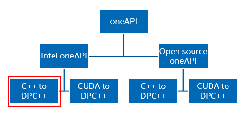
Figure 1. oneAPI tree diagram
Since its release, oneAPI has quickly proliferated among companies, universities, and institutions.8 oneAPI’s cross-architectural nature provides unified programming across heterogenous systems and allows ease of code portability and maintenance. The relevance for oneAPI in medical applications lies with the processing system of many medical imaging devices that computes and outputs the 2D and 3D images that are familiar to most people. A recent influx of GPUs for data processing in the medical device market has led to a mix of CPUs and GPUs in processing systems.9 These heterogeneous systems are what oneAPI is intended to target, so customers can focus more on optimizing performance across hardware and less on maintaining multiple code bases for multiple devices.
The primary language for oneAPI is DPC++10 (based on C++ and SYCL* standards) that when used in correspondence with a set of libraries for API-based programming allows for the code reuse that oneAPI supports.
The rest of this paper focuses on implementation, specifically the process of migrating a program originally written in C++ to DPC++ and running it on Windows.
C++ to DPC++ Migration: oneAPI Parallel Implementation of Convolution
DPC++ can be understood as an extension to the C++ language that allows a program to access parallel computing functionalities with a heterogeneous system (similar to SYCL). It includes devices such as CPUs, GPUs, and FPGAs. Therefore, migrating C++ to DPC++ means simply adding details to support parallelism in the program.11 Remember that the goal of parallelism is to compute things faster by running multiple tasks at once, thereby increasing throughput and reducing latency.
An earlier white paper reviews the use of 2D fast Fourier transform (2D FFT) and convolution for medical image reconstruction. This paper uses C++ code from the earlier paper to demonstrate migration to DPC++. While the process of migration may differ based on the specifics of every program, the general steps, validated on Windows-based systems (for details, see the Configurations section), are as follows:
Step 1: Install the Base Kit
The Base Kit works with either Microsoft Visual Studio* 2017 or 2019 , so if you are planning to use Visual Studio, ensure that one of these versions is installed prior to installing the Base Kit.
To run oneAPI code samples on Windows:
- Install the latest version of oneAPI. If the system already has an older version of oneAPI installed, it is recommended to uninstall the older version first. To do this: In the Start menu, search for add or remove programs, scroll down to oneAPI Basic Toolkit, and then select Uninstall. Then reinstall the newest version. Download the Base Kit12
- Ensure the system is using the latest graphics driver for the Base Kit. Download the Graphics Driver13
The next step is not necessary for a migration set up but can be used to ensure a proper set up in the Visual Studio environment.
Under the Extensions tab, select Intel/Browse Intel oneAPI Samples. When the window appears, select Base Vector Add14 and then OK. Successfully running this project means the environment is set up correctly using Intel® oneAPI DPC++/C++ Compiler.
- In the Solution Explorer window, right-click the project, and then select Properties.
- Go to Configuration Properties/General and make sure that the Platform Toolset is set to Intel® oneAPI DPC++/C++ Compiler.
- Go to the Build tab and select Build Solution. This compiles the project cleanly.
- Go to the Debug tab and select Start Debugging. If the run is successful, the terminal window matches what's shown in Figure 2:
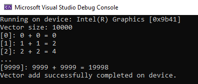
Figure 2. Successful run of a vector-add sample
Step 2: Identify Opportunities for Parallelism
After successfully installing the Base Kit and setting up a DPC++ workspace, it is time to return to migrating the desired program. The easiest way to approach adding parallelism to a program is to identify an isolated point in the code with the greatest parallelism potential, work on it, and then branch out from there. In this case, convolving the image with the filter requires iterating through every pixel in the image. Each repetition of the same operation on every piece of data runs independently of others, making this a great location to apply parallelism. The following code snippet shows the original brute force convolution method (notice the nested for-loops):
//function that runs the brute force convolution on the image

void brute_force_2d_convolution(int kCols, int kRows, float* input_image, float* out_image, float* kernel, int img_height, int img_width) {

    // find center position of kernel (half of kernel size)
    int kCenterX = kCols / 2;
    int kCenterY = kRows / 2;
    // Since the image is laid out columns first and then rows, we can just set this to 0 for the 0,0 location
    // and increment it each time through the outer loops to access the next pixel value
    int img_index = 0;

    // Work through each row of the input_image
    for (int row = 0; row < img_height; ++row)
    {
        // Work through each column of the input_image
        for (int col = 0; col < img_width; ++col)
        {
            // Since the kernel is laid out columns first and then rows and convolution uses the flipped kernel
            // we will start with the last pixel location (e.g., 4, 4 for a 5x5 kernel) and work backwards
            // decreasing the index each time through the inner loops.
            int kern_index = (kRows * kCols) - 1;

            // When convolving there are many options on how to handle the outer edge pixels where the kernel does
            // not fit fully over the image.  This algorithm opts to return an output image that is the same
            // size as the input image, but sets all the border pixels where the kernel is not fully over the image
            // to black (0.0).

            if (col < kCenterX || col + kCenterX >= img_width || row < kCenterY || row + kCenterY >= img_height)
            {
                out_image[img_index] = 0.0f;
            }
            else
            {
                // Work through each row of the kernel image
                for (int kRow = 0; kRow < kRows; ++kRow)
                {
                    // Calculate the index into the provided image where the kernel upper left corner
                    // would start on the image for the row,col pixel convolution
                    int conv_index = (row - kCenterY + kRow) * img_width + col - kCenterX;

                    // Work through each column of the kernel image
                    for (int kCol = 0; kCol < kCols; ++kCol)
                    {
                        out_image[img_index] += input_image[conv_index] * kernel[kern_index];

                        kern_index--;
                        conv_index++;
                    }
                }
            }

            img_index++;
        }
    }
}
The key to data-parallel programming is to effectively distribute the workload over computational resources at hand. In this case, there is no reason to wait for a single device to linearly run 262,144 convolutions (for a 512 x 512 image) when multiple threads can be used at once.
Step 3: Incorporate DPC++ Components
After identifying the desired parallelisms to the existing code, most of the C++ code can remain the same but with the addition of a few key DPC++ components.15 For more information regarding DPC++ components such as platforms, devices, queues, buffers, accessors, and more, see chapters 1 and 3 of Data Parallel C++: Mastering DPC++ for Programming of Heterogeneous Systems Using C++ and SYCL.16
- Use a device selector abstraction to specify a device on which a queue runs (using the device_selector class). The following is an example of a generic device selector that chooses an available device behind the scenes, as well as the setup for an FPGA emulator. You also have the capacity to specify the kind of device (CPU, GPU, FPGA) by changing the line that says configurable_device_selector dselector to cpu_selector dselector or gpu_selector dselector, for example.
//************************************ // Function description: create a device queue with the default selector or // explicit FPGA selector when FPGA macro is defined // Return: DPC++ queue object //************************************ queue create_device_queue() { // create device selector for the device of your interest #ifdef FPGA_EMULATOR // DPC++ extension: FPGA emulator selector on systems without FPGA card intel::fpga_emulator_selector dselector; #elif defined(FPGA) // DPC++ extension: FPGA selector on systems with FPGA card intel::fpga_selector dselector; #else // the default device selector: it will select the most performant device // available at runtime. // similarly, the code can be run on GPU by uncommenting the gpu_selector line // below instead of using the cpu_selector. cpu_selector dselector; //default_selector dselector; //gpu_selector dselector; #endif // create an async exception handler so the program fails more gracefully. auto ehandler = [](cl::sycl::exception_list exceptionList) { for (std::exception_ptr const &e : exceptionList) { try { std::rethrow_exception(e); } catch (cl::sycl::exception const &e) { std::cout << "Caught an asynchronous DPC++ exception, terminating the " "program." << std::endl; std::cout << EXCEPTION_MSG; std::terminate(); } } }; try { // create the devices queue with the selector above and the exception // handler to catch async runtime errors the device queue is used to enqueue // the kernels and encapsulates all the states needed for execution queue q(dselector, ehandler); return q; } catch (cl::sycl::exception const &e) { // catch the exception from devices that are not supported. std::cout << "An exception is caught when creating a device queue." << std::endl; std::cout << EXCEPTION_MSG; std::terminate(); } } - Create buffers to store the data that needs to be shared between the host and the devices. This example needs a buffer to hold the filter, the input image, and the output image after convolution.
- Create accessors to interact with the memory in the buffers. Accessors can be created with permission to read, write, or read-write the data in a specific buffer (they are the only way to access memory in a buffer). A read-only accessor copies the data to the device but does not copy the data back to the host. A write-only accessor copies the data back from the device to host once the kernel is done but does not copy data to the device. This optimizes data transfers if all data stored in the buffer is computed from other data. A read-write accessor transfers data both ways.
- Create a queue and submit a kernel to the queue.
- Call parallel_for to run convolutions on device in parallel. Similar to depends_on(), parallel_for() is also a function the Intel® oneAPI Toolkit provides. It appears in most DPC++ programs. This example of parallel_for() uses parameters col and row to iterate through each column and row value in order to access every individual pixel in the image, but it is ultimately up to programmer discretion on the receiving variable names. The example code uses col and row to determine the location the the specific pixel and then convolves it with the filter, all within the parallel_for() call.
The code snippet below covers steps 2 and 3.
//************************************
// Compute brute force convolution DPC++ on device: convolved image is returned in
// 4th parameter "output_image"
//************************************
void BruteForceConvolutionInDPCPP(int kCols, int kRows, float *input_image, float *output_image,
    float *kernel, int img_height, int img_width) {

    try {

        // print out the device information used for the kernel code
        std::cout << "Device: " << q.get_device().get_info<info::device::name>()
            << std::endl;

        // create the range object for the arrays managed by the buffer
        size_t num_pixels = img_height * img_width;

        // create buffers that hold the data shared between the host and the devices.
        //    1st parameter: pointer of the data;
        //    2nd parameter: size of the data
        // the buffer destructor is responsible to copy the data back to host when it
        // goes out of scope.
        buffer kernel_buf(kernel, range(kCols* kRows)); //use kernel size not image size
        buffer input_image_buf(input_image, range(num_pixels));
        buffer output_image_buf(output_image, range(num_pixels));

        // submit a command group to the queue by a lambda function that
        // contains the data access permission and device computation (kernel)
        q.submit([&](handler& h) {
            // create an accessor for each buffer with access permission: read, write or
            // read/write the accessor is the only mean to access the memory in the
            // buffer.
            accessor kernel_accessor(kernel_buf, h, read_only);
            accessor input_image_accessor(input_image_buf, h, read_only);

            // the output_image_accessor is used to store (with write permision) the output image data
            accessor output_image_accessor(output_image_buf, h, write_only);

            // Use parallel_for to run convolution in parallel on device. This
            // executes the kernel.
            //    1st parameter is the number of work items to use
            //    2nd parameter is the kernel, a lambda that specifies what to do per
            //    work item. the parameter of the lambda is the work item id of the
            //    current item.
            // DPC++ supports unnamed lambda kernel by default.
            h.parallel_for(range<2>(img_width, img_height), [=](id<2> idx) {
                // find center position of kernel (half of kernel size)
                int col = idx[0];
                int row = idx[1];
                int kCenterX = kCols / 2;
                int kCenterY = kRows / 2;
                int img_index = row * img_width + col;

                // When convolving there are many options on how to handle the outer edge pixels where the kernel does
                // not fit fully over the image.  This algorithm opts to return an output image that is the same
                // size as the input image, but sets all the border pixels where the kernel is not fully over the image
                // to black (0.0).

                if (col < kCenterX || col + kCenterX >= img_width || row < kCenterY || row + kCenterY >= img_height)
                {
                    output_image_accessor[img_index] = 0.0f;
                }
                else
                {
                    // Since the kernel is laid out columns first and then rows and convolution uses the flipped kernel
                    // we will start with the last pixel location (e.g., 4, 4 for a 5x5 kernel) and work backwards
                    // decreasing the index each time through the inner loops.
                    int kern_index = (kRows * kCols) - 1;

                    // Work through each row of the kernel image
                    for (int kRow = 0; kRow < kRows; ++kRow)
                    {
                        // Calculate the index into the provided image where the kernel upper left corner
                        // would start on the image for the row,col pixel convolution
                        int conv_index = (row - kCenterY + kRow) * img_width + col - kCenterX;

                        // Work through each column of the kernel image
                        for (int kCol = 0; kCol < kCols; ++kCol)
                        {
                            output_image_accessor[img_index] += input_image_accessor[conv_index] * kernel_accessor[kern_index];

                            kern_index--;
                            conv_index++;
                        }
                    }
                }

            });

        });

        // q.submit() is an asynchronously call. DPC++ runtime enqueues and runs the
        // kernel asynchronously. at the end of the DPC++ scope the buffer's data is
        // copied back to the host.
        q.wait();
    }
    catch (sycl::exception& e) {
        // Do something to output or handle the exception
        std::cout << "Caught sync SYCL exception: " << e.what() << "\n";

        std::terminate();
    }
    catch (std::exception& e) {
        std::cout << "Caught std exception: " << e.what() << "\n";
        std::terminate();
    }
    catch (...) {
        std::cout << "Caught unknown exception\n";
        std::terminate();
    }
}
Note For this DPC++ syntax, compile it with ISO C++ 17 Standard (/std:c++17) or a later version. To check the version, in the Solution Explorer panel, right-click the project, and then go to Properties/DPC++/Language/C++ Language Standard.
The convolution code written in DPC++ in its entirety can be found on GitLab*. Additional DPC++ example programs can be found on GitHub*17.
Sample Output
When run with the command line arguments --operation=blur --kernel_size=5 --repetitions=11 head_ct.png, both the original C++ and new DPC++ convolution program are expected to return the same resultant image. To sharpen an image instead of blurring it, blur can be replaced with sharpen. Figure 3 shows example outputs of the program run using an image of a brain from a CT scan:
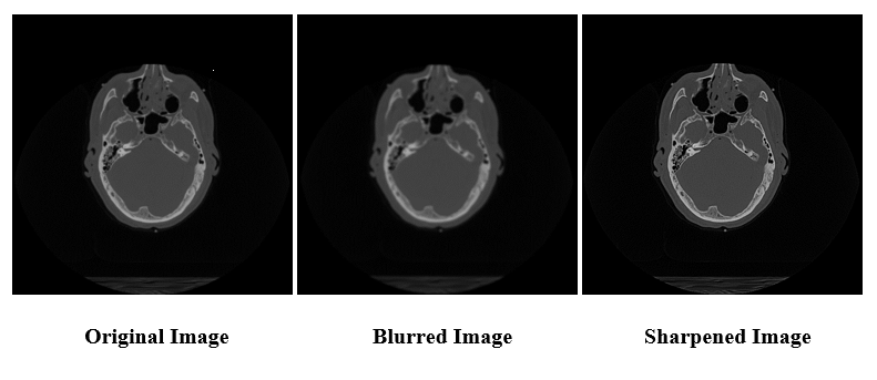
Figure 3. Original image vs. output images
Comparison of Results
This section compares the results of the C++ (regular) with the DPC++ (parallel) implementation of the convolution code along the bases of performance and accuracy. The regular convolution runs on the CPU host device (Intel® Core™ i7-10610U processor), and the parallel convolution runs on multiple threads on the integrated GPU (iGPU [Intel® UHD Graphics]). For more details, see the system configuration section.
Performance
The code is set up to allow the program to run both the regular and parallel convolution 10 times and print the minimum, maximum, and average runtimes. When it first ran, the parallel method took roughly 1.00 seconds per run while the regular convolution only took approximately 0.065 seconds per run. The authors investigated this runtime, as the parallel programming that DPC++ allows is expected to display improved runtimes. Intel® VTune™ Profiler18 is an incredibly useful tool for optimizing system performance and is compatible with DPC++. Figure 4 shows a screenshot of the Intel VTune Profiler analysis on a run of the program:

Figure 4. Intel VTune Profiler results for initial parallel convolution implementation
The Intel VTune Profiler results show ten runs of the program on both the CPU and integrated GPU, respectively. The blue blocks are the clBuild times for the kernel, and the peach blocks are the runtimes for the convolution calculations. As shown by the Intel VTune Profiler, the GPU runs faster, however, even within that, the kernel build times appeared to take up at least 80 percent of the total time (with each build taking about 0.5s).
After further investigation, the authors realized that the queue was getting initialized within the BruteForceConvolutionInDPCPP() function that ran 10 times to find the average runtime. When working with oneAPI for the first time, it is reasonable to want to initialize the queue in the same function as the parallel_for() call. However, this prevents the program from caching the build and the ability to reuse the same queue for subsequent calls. As a result, Intel VTune Profiler results display 10 separate clBuilds for the 10 runs of the convolution.
To resolve this issue, the authors moved the declaration of the queue to a higher level scope (currently a global variable but could just as easily be a local variable in main) to ensure that it would not get destroyed each time the subfunction ended and the queue went out of scope. With this new structure, the queue is not destroyed and caches the kernel's build results. It later reuses the previously built kernel on subsequent calls. Figure 5 shows the Intel VTune Profiler results for the updated code.

Figure 5. Intel VTune Profiler results for revised parallel convolution implementation
Notice how there is now only one blue clBuild block that occurs before all the runs on a specific device. After this change, the convolution runtimes of the DPC++ implementation are more comparable to the original runtime. Figure 6 shows the runtime results of the regular convolution, and Figure 7 shows the runtime results for the convolution run in parallel using DPC++:
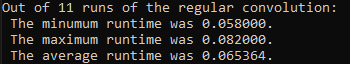
Figure 6. Runtime results of regular convolution
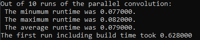
Figure 7. Runtime results of parallel convolution
The average runtime for the parallel convolution is calculated over 10 runs, not including the very first run with the clBuild. This is because as the size of the media increases to video frames or another type of streaming data, the startup cost of the one-time build becomes less relevant in comparison. In other words, for convolving an image as small as the one used in this sample, the overhead for building the queue may arguably outweigh the benefits of parallel computing, but as the media size increases, parallel programming becomes more worthwhile. Another option to further optimize the runtime is to use the DPC++ ahead-of-time (AOT) compilation19 that builds all of the necessary components before actually running the program. This also comes with its own set of tradeoffs, such as additional hardware specifications and increased load time, so the decision to use AOT compilation or just-in-time (JIT) compilation is ultimately up to you.
For these reasons, the authors decided to factor out the clBuild time when using DPC++ compiler and only compare the pure computational runtimes of both the regular and parallel convolution. The regular convolution took approximately 0.065 seconds, and the parallel convolution took about 0.079 seconds. While the difference in this case is minimal, the payoff for parallel computing grows alongside the size of the media it is being applied to.
Accuracy
Parallel computing should maintain the same degree of accuracy as the original implementation. More specifically, when the parallel convolution runs on a CPU, it returns the exact output image, to the pixel, as the regular convolution run on the host. On the other hand, when the parallel convolution runs on the integrated GPU (iGPU), the output image may differ slightly. This is simply due to slight differences in the way that CPUs and iGPUs handle floating-point numbers that lead to minor rounding differences. In this case, the occasional difference in pixel values is expected and negligible, if noticeable in the image at all. Within the program, accuracy is checked with a for-loop that iterates through each pixel in the image and compares the corresponding value of the output image from the parallel convolution with the expected output image from the regular convolution. For the iGPU results in this case, 237,854 out of 262,144 pixels were identical (90.7 percent), and for those that differed, the maximum difference between pixel values was 0.000031.
Additional Considerations
While this paper covers basic considerations for C++ to DPC++ migration, the authors propose using Unified Shared Memory (USM) as an extension to the previously reviewed code. In this way, the host and device can share a pointer value to access the same shared memory. When using USM with a CPU and integrated GPU, no memory copying is necessary. On the other hand, using USM with a CPU and discrete GPU (dGPU) requires making a copy of the data since the dGPU does not share memory with the CPU complex. While you do not need to worry about doing this since USM takes care of it, it is still valuable to understand how USM timing expectations may vary based on devices.
Currently the program uses buffers and accessors to access the data from devices other than the host, but since the example code was run on an iGPU, USM could be used instead to avoid redundant copies of the image data. In fact, USM is a more intuitive way of handling data when converting C++ to DPC++ than the use of buffers and accessors. Broadly speaking, it involves little more than a call to the function malloc_shared() for memory allocation and adding in a wait() call at the end of the parallel_for() call. oneAPI with USM Samples on GitHub20
An additional consideration when choosing to use USM (that applies broadly to parallel computing) is dependencies within the code. For example, if the success of task B relies on the completion of task A, task B is dependent on task A. When working with queues (whether in order or out of order) that direct tasks to each device, pay attention to the runtime of tasks, as the program may need to wait (see function wait()) for one task to complete in order to continue running effectively. The Base Kit includes a function depends_on() that allows you to specify dependencies between events.

Figure 8. Dependency chart from Data Parallel C++: Mastering DPC++ for Programming of Heterogeneous Systems Using C++ and SYCL, 7921
The authors would also like to highlight Intel DevCloud for oneAPI22 as an alternative to running code on a local system. Intel® DevCloud for oneAPI is a remote development environment running oneAPI that gives you access to Intel's latest hardware and software. In this way, you can experiment with DPC++ in the context of heterogeneous environments.
Conclusion
Migrating a program from C++ to DPC++ mainly involves adding parallel computing components, such as queues, buffers, and accessors, to maximize use of available hardware. This paper explores the application of oneAPI programming on a non-AI healthcare example and highlights the potential for performance enhancement. The capabilities of oneAPI extend far beyond those demonstrated in the example code, but this paper is intended to help you set up and become more familiar with the oneAPI DPC++ and C++ compiler work environment.
References
- Fast Fourier Transform (FFT) and Convolution in Medical Image Reconstruction
- Open-Source oneAPI
- Khronos Group
- Gold Release of Intel oneAPI Toolkits Arrive in December: One Programming Model for a Heterogeneous World of CPUs, GPUs, and FPGAs
- Intel oneAPI Base Toolkit
- Programming Guide: Migrating from CUDA to DPC++
- Intel® DPC++ Compatibility Tool
- Intel oneAPI Reviews
- Fujifilm VisualSonics* Accelerates AI for Ultrasound with Intel
- DPC++
- Intel® oneAPI DPC++ Library
- Get the Intel oneAPI Base Toolkit
- Graphics Driver for the Base Toolkit Now Available
- Code Sample: Vector Add–An Intel® oneAPI DPC++/C++ Compiler Example
- DPC++ Components
- Master DPC++ for Programming of Heterogeneous Systems Using C++
- Data Parallel C++ samples
- Intel VTune Profiler
- AOT Compilation
- oneAPI USM Samples on GitHub
- Master DPC++ for Programming of Heterogeneous Systems Using C++
- Intel DevCloud for oneAPI
General References
The code in this article is copyrighted © 2021 Intel Corporation under SPDX-License-Identifier: MIT.
Configurations
The sample codes and analysis were run on a system with following configurations: Intel Core i7-10610U processor, Intel UHD Graphics, 16 GB DDR4-2666 SDRAM. Operating System: Windows 10 Enterprise. Running: Base Kit 2021.3 and graphics driver for the Base Kit (version 26.20.100.7463).