Abstract
Diffusion-weighted imaging (DWI) is a type of magnetic resonance (MR) imaging that uses the diffusion of water molecules to image patterns of the diffusion process of molecules. These diffusion patterns can reveal details about certain possible pathologies in tissue.
DWI signals can be simulated using Monte Carlo simulation, where trajectories of randomly moving water molecules are tracked through an arrangement of cells (represented by simple geometric objects like spheres or cubes).
In this tutorial, an example of a Monte Carlo simulation of diffusion of water molecules in tissue is used to show a vectorization methodology on Intel® Xeon® Scalable processors. The Monte Carlo simulation used here is based on research done at Oregon Health & Science University (OHSU)1, 2, and it can be modified to more complex simulations of DWI.
We show that the trajectories for several particles (water molecules in this case) can be computed simultaneously in Single Instruction Multiple Data (SIMD) mode, instead of computing just one particle at a time. This rearrangement of the code introduces some data dependencies that might prevent automatic vectorization. We show a way to reduce the impact of conditional structures and dependencies so the compiler can automatically vectorize the code. Profiling the code using tools from the Intel® Parallel Studio suite will also be shown.
Introduction
Computer modeling and simulations of biological systems, also called in silico experiments, are an important tool for understanding biological phenomena. A biological model, which is an abstraction of the real biological system under study, is defined. A simulation algorithm is also used to simulate the model’s temporal evolution.
In this article, we present a simple example of a Monte Carlo simulation of the diffusion of water molecules in tissue. This kind of computational experiment can be used to simulate acquisition of a diffusion signal, which is the base of diffusion magnetic resonance imaging (dMRI). This example is based on simulations and research performed at the Advanced Imaging Research Center at OHSU1, 2. We thank OHSU for their permission to publish this article and the source code (available to download) as an educational resource for code modernization efforts.
Problem Statement
The model for the simulation consists of water molecules moving through a 3D array of cells in a tissue sample (water molecule diffusion). In this article, we use a uniform rectilinear 3D array of digital cells, where cells are spaced regularly along each direction (Figure 1).
One possible way to model the cells in the grid is to use spherical cells, where each cell is modeled by a sphere of radius R (which is constant across the 3D grid). Figure 1 shows the grid layout (for simplicity, a 2D grid is shown here, although the grid for the simulation has a 3D structure). Cells, represented as green circles (spheres in our simulation) with radius R, are located in the center of each grid cell.

Figure 1. Grid structure for simulation using spheres (left) and a single cell of radius R(right).
A more general way to represent the cells would be to use a variable 3D shape that can vary from a sphere to a cube (Figure 2). This way the ratio of volumes used by cells and plasma can vary for different simulations. In this tutorial, we use a hyperellipsoid that has a shape that can vary from spherical to cubic, according to a cubicity parameter cp. In this case, the distance R between the center of the cell and the cell boundary (a constant radius R in the case of a sphere) is given by the following expression3:
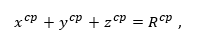
where hyperellipsoid coordinates
are used. θ and φ are the polar and azimuthal angles, respectively α1, α2 and α3 are the axes of the hyperellipse.
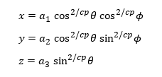
Cell shapes are controlled by parameter CP (Cubicity)
Depending on the value of CP, cell shape can vary from sphere to cube (depicted in 2D here)
Bottom image in 3D
Figure 2. Grid structure for simulation using hyperellipsoids.
Water molecule diffusion is simulated by defining particles P (simulated water molecules) at random positions in the grid, followed by random walks of these particles in the ensemble of cells in the grid (Figure 3). During the random walks, particles can move randomly inside or outside simulated cells. To control the flux of particles through cell membranes, a permeability parameter P is used ¹. The positions of these particles at every time step in the simulation, the number of times they go through a cell membrane (in/out), as well as the time every particle spends inside and outside cells is recorded. These measurements are a simple example of useful information that can be used to simulate an MR signal, which we use in this article to illustrate examples of computations that can possibly prevent automatic vectorization in the simulation code.

Figure 3. Random walks of particles (simulated water molecules) in the ensemble of cells in the grid.
Base Algorithm and Code
A straightforward algorithm to perform the simulation is shown in Figure 4. Starting with a grid that contains only cells, a particle is created at a random position in the grid. This particle is randomly moved at each time step. The location of the particle is recorded at the end of every time step. This step is repeated until the end of the simulation time for this particle is reached (N time steps).
The steps above are repeated for every new particle in the simulation until the number of simulated particles is reached (M particles). Following is a pseudocode for the base algorithm shown in Figure 4.
For each particle (1 .. M)
      For each time step (1 .. N)
	  1. Move particle
	  2. Locate particle (in/out cell, cell number)
	  3. Gather statistics
       End
End
Figure 4. Base algorithm.
The following code section shows fragments of the base code, presenting the two loops shown in the base algorithm in Figure 4.
	(…)
 55 int main() {
 56     float SD = 0.33;
 57     int nsteps = 10000;
 58     float a = 0.0;
 59     float b = 1.0;
        (…)
 99     for (int i = 0; i < NMOLECULES; i++) {
100         error_code = vsRngGaussian(METHOD, stream, 3 * nsteps, normal_rng_buffer, a, b);
101         CheckVslError(error_code);
102         error_code = vsRngUniform(METHOD, stream, nsteps, uniform_rng_buffer, a, b);
103         CheckVslError(error_code);
104
            (…)
127         for (int step = 0; step < nsteps; step++) {
128             mcurr[0] = m[0] + (normal_rng_buffer[3*step] * SD);
129             mcurr[1] = m[1] + (normal_rng_buffer[(3*step) + 1] * SD);
130             mcurr[2] = m[2] + (normal_rng_buffer[(3*step) + 2] * SD);
131
                (…)
195            }
196        }
         (…)
Base Code Analysis
This section describes how to complete a basic performance analysis of the base code using the Intel® C++ Compiler and Intel® Advisor, which are part of the Intel® Parallel Studio XE 2018.
As a first step, we can compile the base code using the Intel C++ Compiler as follows (This command is for demonstration purposes only. Linux* Makefiles to compile the sample code are included in the downloadable zip file):
icc -std=c99 -Wall -g -O3 -xCORE-AVX512 -qopt-zmm-usage=high … -qopt-report=5 -qopt-report-phase=vec
Notice that we have included the option that asks the compiler to generate an optimization report containing vectorization information with the maximum level of information (levels range from 1–5).
Next is a section of the optimization report containing information about the nested loops in the source code.
Begin optimization report for: main()

     Report from: Vector optimizations [vec]

 LOOP BEGIN at baseline.c(99,5)
    remark #15541: outer loop was not auto-vectorized: consider using SIMD directive

    LOOP BEGIN at baseline.c(127,9)
       remark #15344: loop was not vectorized: vector dependence prevents vectorization
       remark #15346: vector dependence: assumed ANTI dependence between
                      num_membrane_interactions[i] (142:21) and num_membrane_interactions[i](142:21)
       remark #15346: vector dependence: assumed FLOW dependence between num_membrane_interactions[i]
                      (142:21) and num_membrane_interactions[i] (142:21)
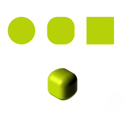
As indicated in the fragment of the report above, the inner loop (loop over time steps) was not vectorized due to data dependencies present. These dependencies are the result of the sequential nature of the time loop in the code, where the computation performed at every iteration depends on the position of the water molecule at the previous time step (Figure 5), which prevents several time steps from being computed simultaneously.
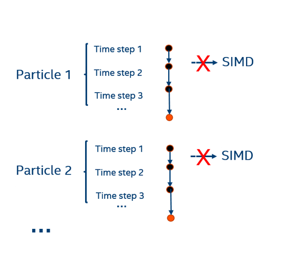
Figure 5. Loop over time steps cannot be vectorized. The computation performed at every iteration depends on the position of the water molecule at the previous time step, which prevents several time steps from being computed simultaneously in vector mode.
Improved Algorithm and Code
To increase opportunities for automatic vectorization, the base code has been modified using the following steps:
- The first step is to perform loop interchange. The variable used in the inner loop (time steps) is switched to the outer loop, and the variable used in the outer loop (particles) is switched to the inner loop. Following is a pseudocode showing the new loop structure.
For each time step (1 .. N)
      For each particle (1 .. M)
	  1. Move particle
	  2. Locate particle (in/out cell, cell number)
	  3. Gather statistics
    End
End
The reason for the loop interchange is that the inner loop in the base code (loop over time steps) cannot be vectorized because it is not possible to compute several iterations of the time loop simultaneously; the position of the particles at a certain time step depend on the position of the particles at the previous time step, as shown in Figure 5.
After the loop interchange, the inner loop (which is now the computations of trajectories of different particles) has a better chance for vectorization because the different particles move independently from each other. - The computation of counters has been modified in the base code. Instead of using conditionals to test the position of the particles (for example, to test if they are inside or outside a cell), Boolean expressions have been introduced (predicates). These Boolean expressions test the position of the particle with respect to the cells by subtracting vectors representing the positions of the particles and cell boundaries with respect to the cell centers (Figure 6). Following is a pseudocode showing the above procedure.
1. Search for the grid cell the particle is currently in
2. Determine if the particle is inside or outside that cell using vector algebra: CB>CP ?
3. Store results (in/out, cell number)
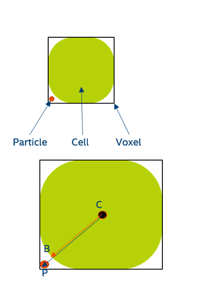
Figure 6. A modified algorithm is used to test if particles are inside or outside cells. No explicit conditional statements are used.
The following code section shows fragments of the improved code. Notice the changes in the loops order which now follow the improved algorithm in Figure 7.
	(…)
 35 int main() {
 36     float SD = 0.33;
 37     int nsteps = 10000;
 38     float a = 0.0;
 39     float b = 1.0;
        (…)
125     for (int step = 0; step < nsteps; step++) {
126         error_code = vsRngGaussian(METHOD, stream, 3 * NMOLECULES, normal_rng_buffer, a, b);
127         CheckVslError(error_code);
128
129         error_code = vsRngUniform(METHOD, stream, NMOLECULES, uniform_rng_buffer, a, b);
130         CheckVslError(error_code);
131
            (…)
133         for (int i = 0; i < NMOLECULES; i++) {
134             mcurr[0][i] = m[0][i] + (normal_rng_buffer[(3 * i)] * SD);
135             mcurr[1][i] = m[1][i] + (normal_rng_buffer[(3 * i) + 1] * SD);
136             mcurr[2][i] = m[2][i] + (normal_rng_buffer[(3 * i) + 2] * SD);
137
               (…)
185            }
186        }
         (…)
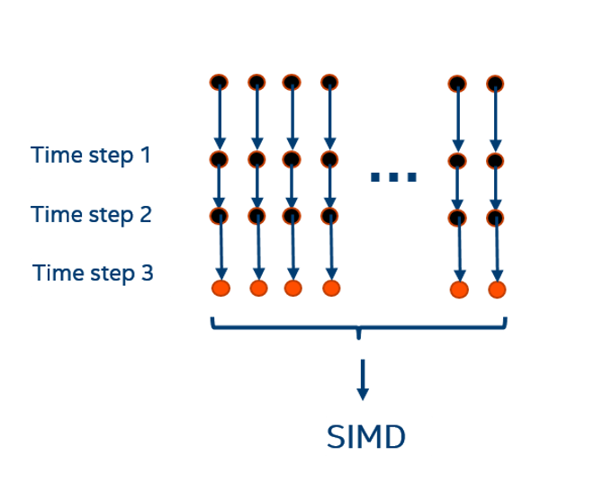
Figure 7. Improved algorithm and vectorized inner loop.
Improved Code Analysis
As we did when analyzing the base code, we start the analysis of the improved code by compiling the code with the options shown next:
icc -std=c99 -Wall -g -O3 -xCORE-AVX512 -qopt-zmm-usage=high … -qopt-report=1 -qopt-report-phase=vecNext is a section of the optimization report showing information about the restructured loops in the improved code.
	LOOP BEGIN at main.c(125,5) remark #25460: No loop optimizations reported

    LOOP BEGIN at main.c(133,9)
    <Peeled, Distributed chunk1>

       LOOP BEGIN at main.c(133,9)
       <Peeled, Distributed chunk1>
          remark #15301: PARTIAL LOOP WAS VECTORIZED
       LOOP END

       LOOP BEGIN at main.c(133,9)
       <Peeled, Distributed chunk2>
          remark #15301: PARTIAL LOOP WAS VECTORIZED
       LOOP END

       LOOP BEGIN at main.c(133,9)
       <Peeled, Remainder loop for vectorization, Distributed chunk2>
       LOOP END

       LOOP BEGIN at main.c(133,9)
       <Peeled, Remainder loop for vectorization, Distributed chunk1>
          remark #15301: REMAINDER LOOP WAS VECTORIZED
       LOOP END
    LOOP END
 LOOP END
As indicated in the report above, the inner loop has been auto-vectorized by the compiler using loop distribution, which is a technique for program restructuring that consists of breaking up the statements in a single loop into two or more loops. The purpose of this is to transform a complex loop that cannot be vectorized (or which has a low vectorization efficiency) into smaller loops that can be vectorized. Loop distribution can reduce register pressure and improve data cache use (Intel® C++ Compiler 18.0 Developer Guide and Reference). The compiler uses its internal heuristics to distribute the loop. However, it is also possible to add a compiler directive at specific locations in the loop (Intel® C++ Compiler distribute_point).
To get detailed information about the performance gain in the restructured loops, we run the Intel Advisor tool using the following commands:
advixe-cl --collect survey --project-dir ./R01--search-dir src:r=./. -- ./random_walk
advixe-cl --report survey -format=xml --project-dir ./R01 --search-dir src:r=./. -- ./random_walk
advixe-cl --collect tripcounts --project-dir ./R01 --search-dir src:r=./.  -- ./random_walk
advixe-cl --report tripcounts -format=xml --project-dir ./R01 --search-dir src:r=./. -- ./random_walk
The first command above shows how to run the command line interface (CLI) version of the Intel Advisor tool to perform a survey analysis. The survey analysis provides information for identifying how the code is using vectorization and where the hotspots for further analysis are.
The second command above will create an xml-formatted report containing the results of the survey analysis generated by the Intel Advisor tool. Both the analysis information and the report will be in the project directory R01, as specified in the commands.
The last two commands shown above illustrate how, once we have performed a survey analysis, we can re-run the Intel Advisor tool to add more information to the analysis and the reports. In this case, we are running the tripcounts analysis to add information about the number of times loops are executed. This extra information will be added to the analysis contained in the project report R01.
Once this information is generated, we can look at the xml reports generated by the Intel Advisor tool, or we can use Intel Advisor’s graphical user interface (GUI). All the performance information from both the survey and tripcounts analyses will be available in either interface. More information and examples on how to use the Intel Advisor tool to analyze loop performance is in Quick Analysis of Vectorization Using Intel® Advisor and Improve Performance Using Vectorization and Intel® Xeon® Scalable Processors.
Figure 8 shows a section of the Intel Advisor GUI. Estimated performance gain, times, and vector efficiency are indicated in the report. Notice how the loop on line 134 was distributed, with the two distributed loops consuming approximately 60 percent of the total execution time.
This improved code is a first step in the optimization process, where the compiler can vectorize the most time-consuming parts of the code (the time and particle displacement nested loops). Next steps in the optimization workflow can be:
- Cache memory optimization and further dependency analysis
- Multithreading
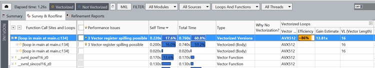
Figure 8. Fragment of Intel® Advisor showing details (including performance gain estimate) for the vectorized loops.
Summary
To make code run faster, software needs to use all opportunities for parallelism that are present in modern hardware. Modern processors offer a larger number of cores and, in each core, width of vector registers is increasing. Intel Xeon Scalable processors support the increasing demands in performance with Intel® Advanced Vector Extensions 512 (Intel® AVX-512), which is a set of new instructions that can accelerate performance for demanding computational workloads.
To take advantage of both multiple cores and wider SIMD units, we need to add vectorization and multithreading to our software. Vectorization in each core is a critical step because of the multiplicative effect of vectorization and multithreading. To get good performance from multiple cores we need to extract good performance from each individual core.
In this tutorial, we describe a methodology to enable auto-vectorization using an example of a Monte Carlo simulation of diffusion of water molecules in tissue. We showed that the trajectories for several particles during the simulation can be computed simultaneously in SIMD mode, instead of computing just one particle at a time. We also showed that the impact of conditional structures and dependencies that arose during the code restructuring can be reduced, so the compiler can automatically vectorize the code.
Our purpose in this tutorial was to show how, even when dealing with a relatively complicated application like a stochastic simulation, simple optimization techniques like loop interchange and use of predicates can allow the application to take advantage of Intel AVX-512 capabilities of the latest generation of hardware, increasing performance significantly.
References
1. C. S. Springer, Using 1H2O MR to measure and map sodium pump activity in vivo, Journal of Magnetic Resonance, vol. 291, pp. 110-126, 2018.
2. G. Wilson, C. Springer, S. Bastawrous and J. Maki, Human Whole Blood 1H2O Transverse Relaxation With Gadolinium-Based Contrast Reagents: Magnetic Susceptibility and Transmembrane Water Exchange, Magnetic Resonance in Medicine, vol. 77, pp. 2015-2027, 2017.
3. P. Calvo Portela and F. Llanes-Estrada, Cubic wavefunction deformation of compressed atoms, 2015.