| File(s): | GitHub |
| License: | MIT |
| Optimized for... | |
|---|---|
| Software: (Programming Language, tool, IDE, Framework) |
Intel® oneAPI DPC++/C++ Compiler |
| Prerequisites: | Familiarity with C++ and DPC++ |
This tutorial with code examples is an Intel® oneAPI DPC++ Compiler implementation of a two-dimensional finite-difference stencil that solves the 2D acoustic isotropic wave-equation. It illustrates the basics of the (Data Parallel C++) DPC++ programming language using direct programming.
Requirements
C++ programming experience and familiarity with the DPC++ basics are assumed. If you do not have prior exposure to DPC++, see the resources listed at the end of this tutorial.
Introduction
In this tutorial, we chose the problem of solving a Partial Differential Equation (PDE) using a finite-difference method to illustrate the essential elements of the DPC++ programming language, including queues, buffers/accessors, and kernels (you can access the code on GitHub*). You can use this tutorial as an entry point to start programming in DPC++ or as a proxy to develop or better understand complicated code for similar problems. For example, a more complex DPC++ code sample implementing a 16th-order finite-difference stencil for the 3D isotropic wave equation is available on GitHub.
PDEs can describe many physical phenomena. One example is the wave equation, which describes waves propagating through a medium with specific characteristics (for example, isotropic or anisotropic, constant or variable density, and so on).
Finite-difference methods approximate the solution of PDEs by approximating the continuous PDEs by a set of discrete difference equations, which can be solved iteratively in a computer.
Other examples of PDEs that finite-difference methods can solve include option pricing (in mathematical finance), Maxwell’s equations (in computational electromagnetics), the Navier-Stokes equation (in computational fluid dynamics), and others. The simple parallel finite-difference method in this example can be easily modified to solve problems in the above areas.
This tutorial provides a DPC++ code sample that implements the solution to the wave equation for a 2D acoustic isotropic medium with constant density. This wave equation is solved using the finite-difference method (a 2nd-order stencil) with the purpose of modeling wave propagation in the medium. This is useful in several disciplines, including earthquake and oil exploration seismology, ocean acoustics, radar imaging, and nondestructive evaluation.1
Problem Statement
If the medium is acoustic and its density is constant, the wave equation (PDE describing wave propagation in the medium) is:
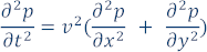
Where p is the pressure, v is the medium velocity (velocity at which acoustic waves propagate in the medium), x and y are the two Cartesian coordinates, and t is the time. The wave can be initiated using initial conditions defined by p at t=0 or an explicit source function s(x,y). This code sample uses an explicit source function.
To obtain an approximate solution to this problem, we divide the model into a grid of N by N points (for simplicity, we use a square grid, but a rectangular grid can be used). If we call ∆x, ∆y the distance between points in the grid in the x and y axes, respectively. If ∆t is the increment in time (where time iterations range from n=0 to a defined maximum number of iterations), then by approximating the continuous partial derivatives using 2nd-order central differences, we obtain the discretized equation:

And solving for  (the value of the pressure wavefield at position i,j at time n+1), we can now describe a finite-difference formula to approximate the solution of the 2D acoustic wave equation:

This is an explicit formula for the values of the pressure wavefield at time n+1 (at every point in the grid) based on the values of the pressure wavefield at time n and n-1.
Parallel Implementation and Code Sample Walk-Through
Grids used to represent models in finite-difference computations are natural candidates for simple domain-decomposition techniques because of their regularity. This is especially evident in the explicit finite-difference scheme shown here. It can be finely partitioned to expose the maximum possible concurrency by defining a task for each grid point because there are no data dependencies when computing the wavefield at different grid points for a given time step. Every point in the grid can be updated independently at every time iteration because the only data dependencies are on neighboring grid points at previous time steps, which are read-only.
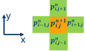
At each time iteration, each point in the 2D grid can be updated according to the explicit formula shown above, as depicted in the following graphic representation of the stencil, where the updated value for the pressure wavefield is orange, and the neighboring grid points used for the update are green:
In this code sample, the update is included in the Iso2dfdIterationGlobal function:
// Stencil code to update grid point at position given by global id (gid)
// New time step for grid point is computed based on the values of the
//    the immediate neighbors in both the horizontal and vertical
//    directions, as well as the value of grid point at a previous time step

value = 0.0;
value += prev[gid + 1] - 2.0f * prev[gid] + prev[gid - 1];
value += prev[gid + n_cols] - 2.0f * prev[gid] + prev[gid - n_cols];
value *= dtDIVdxy * vel[gid];
next[gid] = 2.0f * prev[gid] - next[gid] + value;
main() Function
Now, we look at the main function. Four one-dimensional arrays are defined and allocated, for example:
int main(int argc, char* argv[]) {

  // Arrays used to update the wavefield

  float* prev_base;
  float* next_base;
  float* next_cpu;
  // Array to store wave velocity
  float* vel_base;
Three of these arrays are used to update the wavefield in the kernel function, where prev_base and next_base represent the pressure wavefield at iterations n and n+1, respectively. vel_base stores the medium velocity. The next_cpu array is equivalent to the next_base array, and it validates the computation in the device compared to the same computation performed in the host.
These arrays are allocated and passed as parameters to the initialize function, which initializes the wavefield arrays and velocity array and adds the source function to the prev_base array. The source function used here is a discretized Ricker wavelet, commonly used in seismic data processing:
// Initialize arrays and introduce initial conditions (source)

Initialize(prev_base, next_base, vel_base, n_rows, n_cols);
DPC++ Device Selector, Queues and Buffers
So far, we have used standard C++ code. We start using DPC++ functionality when we create a device queue, which is used to enqueue work that will be executed in a particular device or accelerator.
// Create a device queue

queue q(default_selector_v);
We can create device queues that send work to specific devices. For example, we can use a GPU selector to queue work in a GPU or a default selector, which would select a device at runtime, as shown here.
The next step is creating buffer objects communicating data between the host and the device. The buffers can store collections of elements that can be one, two, or three-dimensional. In this case, we use them to store 1D arrays of floats (we use 1D arrays to represent 2D grids). Buffers are directly connected to how C or C++ stores arrays, so we connect them to the three arrays used in the pressure wavefield update calculation. Data in these buffers can be communicated back and forth between host and device:
buffer next_buf(next_base, range(n_size));
buffer prev_buf(prev_base, range(n_size));
buffer vel_buf(vel_base, range(n_size));
This shows that one buffer is declared for every float array, and a 1D range of n_size elements specifies the size of the buffer:
// Compute the total size of grid

size_t n_size = n_rows * n_cols;
Command Handler and Kernel Definition
At this point, we want to create a loop that will iterate over time steps. This loop will update the value of the pressure wavefield at every grid point:
// Iterate over time steps

for (unsigned int k = 0; k < n_iterations; k += 1) {

    // Submit command group for execution

    q.submit([&](auto &h) {
At every time iteration, you can submit a command group to the device queue created above. The command group includes the kernel function that will be enqueued to the device defined in the queue. This command group takes an h command group handler as a parameter, constructed at run-time, and includes all the requirements for a kernel to execute.
In a previous step, we created buffers in the host to hold the data we wanted to share between the host and the device. Now, we create accessors to access data from the buffers in the device. These accessors act like pointers to memory objects that can be used in the device and are used in kernel functions to communicate data from and to the host via the buffers that were defined above:
accessor next_a(next_buf, h);
accessor prev_a(prev_buf, h);
accessor vel_a(vel_buf, h, read_only);
Note: The access mode of the accessors is read and write for the buffers propagating the wavefield (next_buf and prev_buf) because these buffers are updated at every time step.
The next step is to define the execution range for the kernel function. In this example, we use a two-dimensional range to define a collection of work items (executing instances of the kernel function). Every work item will execute an instance of the kernel function.
The example uses the grid size (given by input arguments n_rows and n_cols) to define the range:
auto global_range = range<2>(n_rows, n_cols);
Each work item in the range is now identified by a value of type <2>, as shown in the next code snippet, where we send work to the device for execution. In DPC++, we can use the parallel_for function to send a kernel function to execute on the device. This kernel function is constructed using C++ lambda functions syntax. In C++ 11 and later, a lambda expression, like the one shown here, defines a function object at the location where it is invoked.
This parallel_for function creates several instances of the kernel function (specified by the global and local ranges). It adds them to the command queue to be executed in parallel in the device:
h.parallel_for(global_range, [=](auto it) {
      Iso2dfdIterationGlobal(it, next_a.get_pointer(),
                                prev_a.get_pointer(), vel_a.get_pointer(),
                                dtDIVdxy, n_rows, n_cols);
    });
The first parameter in the parallel_for function defines the range over which the kernel function will be executed, given by the global range. The second parameter is an index or ID for each kernel invocation. This parameter ensures that every kernel instance executing in the device has a unique identifier.
In the code snippet above, the body of the kernel function defines the code that will be executed in parallel by every instance of the kernel function created by the parallel_for function; in this case, it’s the invocation of the Iso2dfdIterationGlobal() function. This function updates the pressure wavefield at the grid point specified by the parameter it, which uniquely identifies (indexes) the instance of the kernel function executing in the device.
Before we discuss the Iso2dfdIterationGlobal() function, it is important to know why the code contains an if-else statement that effectively swaps the next_a and prev_a accessors at every iteration:
if (k % 2 == 0)
  h.parallel_for(global_range, [=](auto it) {
        Iso2dfdIterationGlobal(it, next_a.get_pointer(),
                                  prev_a.get_pointer(), vel_a.get_pointer(),
                                  dtDIVdxy, n_rows, n_cols);
      });
else
  h.parallel_for(global_range, [=](auto it) {
        Iso2dfdIterationGlobal(it, prev_a.get_pointer(),
                                  next_a.get_pointer(), vel_a.get_pointer(),
                                  dtDIVdxy, n_rows, n_cols);
      });
This is so two arrays can be used for the update instead of three. By swapping the arrays at every iteration, we do not need to allocate a third array to hold the pressure wavefield at time  because that information can be read from the array about to be updated with the wavefield at time
  .
.
The Iso2dfdIterationGlobal() function updates the pressure wavefield at the grid point specified by the parameter it. In this function, see how the local and global indices can be extracted from the parameter it.
void Iso2dfdIterationGlobal(id<2> it, float* next, float* prev,
                               float* vel, const float dtDIVdxy, int n_rows,
                               int n_cols) {
  float value = 0.0;

  // Compute global id
  // We can use the get.global.id() function of the item variable
  //   to compute global id. The 2D array is laid out in memory in row major
  //   order.
  size_t gid_row = it.get(0);
  size_t gid_col = it.get(1);
  size_t gid = (gid_row)*n_cols + gid_col;
The global ID (gid) can be computed in several ways. The above code snippet shows one possible way and uses member functions of the item class.
The final step is to revisit the stencil computation. Using an if statement in the code snippet below, we first need to check that the update computation does not happen in the border of the array. The finite-difference stencil uses the values of neighboring grid points to update a single grid point. Therefore, it is necessary to check that grid points in the border of the array (the halo) are not being updated to avoid segmentation faults.
The constexpr half_length stores half of the stencil size (2 for this sample).
The computation to update a grid point is done using the value of the gid variable as an index. You can see how this is a fine-grain domain decomposition as every instance of the kernel function will update one point in the grid:
// Computation to solve wave equation in 2D
// First check if gid is inside the effective grid (not in halo)
if ((gid_col >= half_length && gid_col < n_cols - half_length) &&
    (gid_row >= half_length && gid_row < n_rows - half_length)) {
  // Stencil code to update grid point at position given by global id (gid)
  // New time step for grid point is computed based on the values of the
  //    the immediate neighbors in both the horizontal and vertical
  //    directions, as well as the value of grid point at a previous time step
  value = 0.0;
  value += prev[gid + 1] - 2.0f * prev[gid] + prev[gid - 1];
  value += prev[gid + n_cols] - 2.0f * prev[gid] + prev[gid - n_cols];
  value *= dtDIVdxy * vel[gid];
  next[gid] = 2.0f * prev[gid] - next[gid] + value;
}
This step finishes the tutorial walk-through. You can download the complete code sample at GitHub.
This code sample is for educational purposes only; it is not optimized to demonstrate the use of DPC++ basic structures explicitly. This code is intended to provide a basic understanding of DPC++ and can be used as a starting point for further code development in DPC++.
Compiling and Running the Code
To compile and execute the code in Linux*, you need to configure the environment for Intel® oneAPI. Run:
source <oneAPI install dir>/setvars.sh
In the directory where the code sample resides, run:
mkdir build
cd build
cmake ..
make -j
To run the executable, run:
make run
Which will run the executable with pre-selected parameters.
You can also execute the code with different parameters as follows:
./iso2dfd 1000 1000 2000
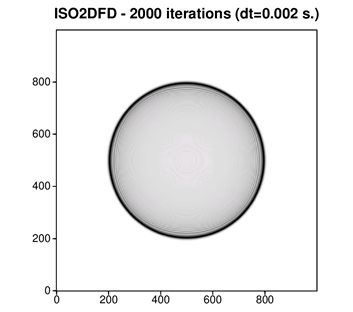
The last command above will run the iso2dfd executable using a 1000x1000 grid size that iterates over 2000 time steps.
The output for the previous execution looks like the wavefield shown in the following figure. It shows a circular wavefront propagating from a source in the middle of the square grid. It was plotted using the output of iso2dfd using the SU Seismic processing library, which has utilities to display seismic wavefields and can be downloaded from John Stockwell’s SeisUnix GitHub* archive.
The following figure shows another example of output. In this case, we define a two-layer model (where the upper portion of the model has an acoustic wave speed of 3000 m/s, and the bottom portion has a speed of 1500 m/s, as shown in the left portion of the figure) and run the code several times varying the total number of time iterations. In this way we can get snapshots of how the wave (and its reflections and refractions at the edges of the model and the interface between the two layers) propagates in time through both the fast and slow portions of the model.

Summary
This tutorial describes a parallel implementation of a two-dimensional finite-difference stencil that solves the 2D acoustic isotropic wave equation. The complete code sample is available to download from GitHub and is intended to show the basic elements of the DPC++ programming language in a simple yet real-world application. You can use this tutorial as a starting point for developing complex applications. In particular, it can help you understand more complex finite-difference stencil parallel codes, like the 3D, 16th-order stencil cited in the Resources section.
Resources
The Intel® oneAPI Toolkits site has detailed descriptions of DPC++ and oneAPI toolkits.
For more documentation and code samples, see Featured Documentation on the Intel® oneAPI Toolkits site.
The ISO3DFD DPC++ code sample is a more sophisticated solution to a 3D isotropic wave propagation problem using a 16th-order stencil.