Train a Apache MXNet* Model in Amazon SageMaker* and Run on IEI Tank* AIoT Developer Kit

Introduction

We will train the Apache MXNet* Gluon model in Amazon SageMaker* to read handwritten numbers of MNIST dataset and then run the prediction for ten random handwritten numbers on IEI Tank* AIoT Developer Kit. More information about IEI Tank* AIoT Developer Kit.

Amazon SageMaker is a platform that enables easy deployment of machine learning models, using Jupyter* Notebooks and AWS* S3 object storage. More information about Amazon SageMaker.

Gluon is a new MXNet library that provides a simple API for prototyping, building, and training deep learning models. We will need MXNet estimator in order to run a MXNet model in Amazon SageMaker. More information about MXNet Gluon models.

Prerequisites

• IEI Tank* AIoT Developer Kit
• Linux* Ubuntu* 16.04 OS
• Python* 2.7
• AWS account

Train a Model

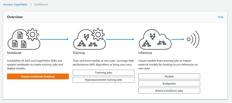
Sign in to your AWS account and go to the Amazon SageMaker.

Create a notebook instance:

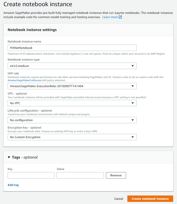
Fill out notebook instance name, add the IAM role, and select Create notebook instance:

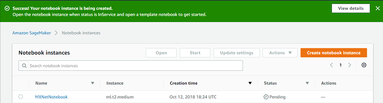
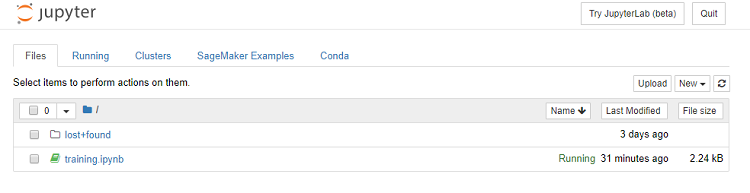
You will see the confirmation on top of the page and the new notebook instance:

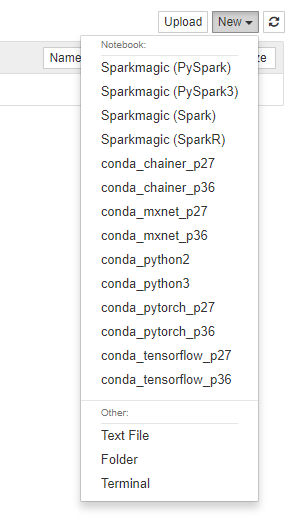
Create a new notebook file by selecting New > conda_mxnet_p27:

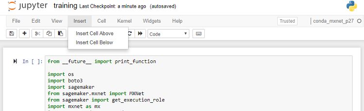
Select Untitled and change the name to training. Select Insert > Insert Cell Below to add cells.

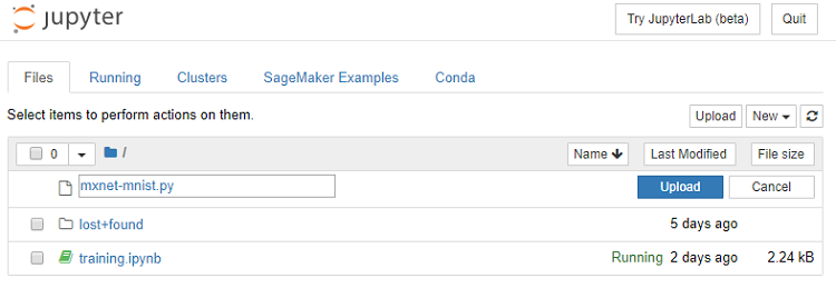
Copy each cell of the Jupyter* Notebook training.ipynb into the cell of your notebook. Find training.ipynb at the end of the tutorial in the Sample Code section. Go to notebook instance and add mxnet-mnist.py (find it in the Sample Code section) by selecting Upload.

Select Upload:

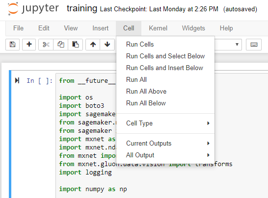
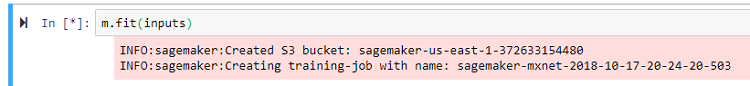
Go back to training.ipynb and run it by selecting Cell > Run All:

Get the information about S3 bucket and training job name:

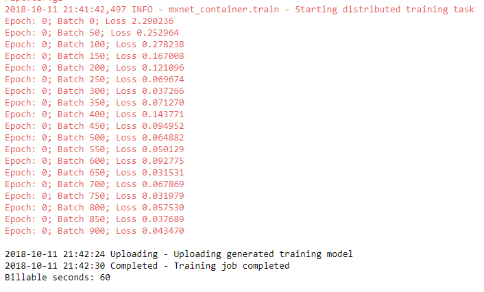
Wait for the all cells to complete running. You will see output similar to this:

Run Prediction

Go to the Amazon S3 > S3 bucket > training job > output:

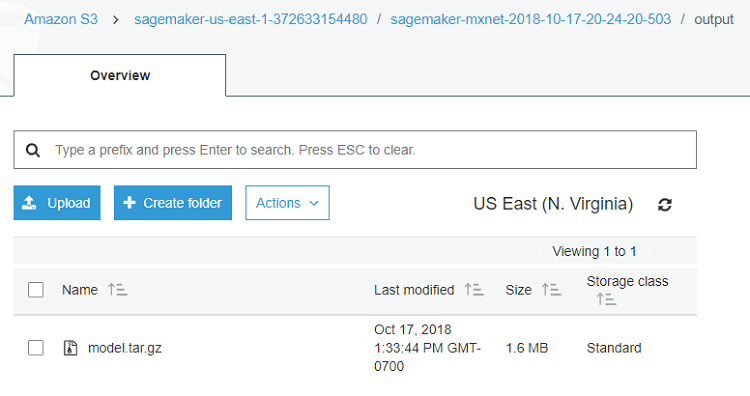
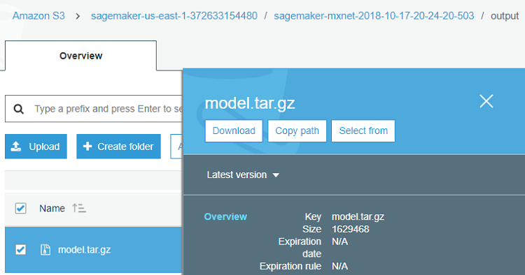
Download the model.tar.gz by clicking on the check box next to it and selecting Download from the right-side menu.

On the Tank, extract the model.params file from the downloaded archive.

tar –xzvf model.tar.gz

If needed, install dependencies.

sudo pip2 install mxnet matplotlib

Save load.py (find it in the Sample Code) in the same folder as model.params.

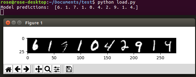
Run load.py:

python load.py

You will see the images of ten random handwritten numbers and the model’s predictions for them:

Conclusion

We have successfully trained the MXNet Gluon model in Amazon SageMaker to read handwritten numbers and got a great prediction for the validation set on Tank.

Sample Code

training.ipynb:

from __future__ import print_function

import os
import boto3
import sagemaker
from sagemaker.mxnet import MXNet
from sagemaker import get_execution_role
import mxnet as mx
import mxnet.ndarray as nd
from mxnet import nd, autograd, gluon
from mxnet.gluon.data.vision import transforms
import logging 

import numpy as np


sagemaker_session = sagemaker.Session()

role = get_execution_role()

gluon.data.vision.MNIST('./data/train', train=True)
inputs = sagemaker_session.upload_data(path='data', bucket='sagemaker-mxnet-gluon')

!cat 'mxnet-mnist.py'

m = MXNet("mxnet-mnist.py",
          role=role,
          train_instance_count=1,
          train_instance_type="ml.c4.xlarge",
          framework_version="1.2.1",
          hyperparameters={'batch_size': 64,
                         'epochs': 1,
                         'learning_rate': 0.001,
                         'log_interval': 100})

m.fit(inputs)

mxnet-mnist.py:

m.fit(inputs)
from __future__ import print_function

import mxnet as mx
import mxnet.ndarray as nd
from mxnet import nd, autograd, gluon
from mxnet.gluon.data.vision import transforms

import numpy as np

import logging
import time


# Clasify the images into one of the 10 digits
num_outputs = 10

logging.basicConfig(level=logging.DEBUG)


# Build a simple convolutional network
def build_lenet(net):    
    with net.name_scope():
        # First convolution
        net.add(gluon.nn.Conv2D(channels=20, kernel_size=5, activation='relu'))
        net.add(gluon.nn.MaxPool2D(pool_size=2, strides=2))
        # Second convolution
        net.add(gluon.nn.Conv2D(channels=50, kernel_size=5, activation='relu'))
        net.add(gluon.nn.MaxPool2D(pool_size=2, strides=2))
        # Flatten the output before the fully connected layers
        net.add(gluon.nn.Flatten())
        # First fully connected layers with 512 neurons
        net.add(gluon.nn.Dense(512, activation="relu"))
        # Second fully connected layer with as many neurons as the number of classes
        net.add(gluon.nn.Dense(num_outputs))

        return net


# Train a given model using MNIST data
def train(channel_input_dirs, hyperparameters, **kwargs):
    ctx = mx.cpu()
    # retrieve the hyperparameters we set in notebook (with some defaults)
    batch_size = hyperparameters.get('batch_size', 64)
    epochs = hyperparameters.get('epochs', 1)
    learning_rate = hyperparameters.get('learning_rate', 0.001)
    log_interval = hyperparameters.get('log_interval', 100)

    # load training and validation data
    # we use the gluon.data.vision.MNIST class because of its built in mnist pre-processing logic,
    # but point it at the location where SageMaker placed the data files, so it doesn't download them again.
    training_dir = channel_input_dirs['training']
    train_data = get_train_data(training_dir + '/train', batch_size)

    # Define the network
    net = build_lenet(gluon.nn.Sequential())

    # Initialize the parameters with Xavier initializer
    net.collect_params().initialize(mx.init.Xavier(), ctx=ctx)
    # Use cross entropy loss
    softmax_cross_entropy = gluon.loss.SoftmaxCrossEntropyLoss()
    # Use Adam optimizer
    trainer = gluon.Trainer(net.collect_params(), 'adam', {'learning_rate': .001})

    # Train for one epoch
    for epoch in range(1):
        # Iterate through the images and labels in the training data
        for batch_num, (data, label) in enumerate(train_data):
            # get the images and labels
            data = data.as_in_context(ctx)
            label = label.as_in_context(ctx)
            # Ask autograd to record the forward pass
            with autograd.record():
                # Run the forward pass
                output = net(data)
                # Compute the loss
                loss = softmax_cross_entropy(output, label)
            # Compute gradients
            loss.backward()
            # Update parameters
            trainer.step(data.shape[0])

            # Print loss once in a while
            if batch_num % 50 == 0:
                curr_loss = nd.mean(loss).asscalar()
                print("Epoch: %d; Batch %d; Loss %f" % (epoch, batch_num, curr_loss))

    return net


def save(net, model_dir):
    # Save the model
    net.save_parameters('%s/model.params' % model_dir)


def get_train_data(data_dir, batch_size):
    # Load the training data
    return gluon.data.DataLoader(
        gluon.data.vision.MNIST(data_dir, train=True).transform_first(transforms.ToTensor()),
                                   batch_size, shuffle=True)

load.py:

from __future__ import print_function

import mxnet as mx
import mxnet.ndarray as nd
from mxnet import gluon
import matplotlib.pyplot as plt

import numpy as np


# Build a simple convolutional network
def build_lenet(net):
    with net.name_scope():
        # First convolution
        net.add(gluon.nn.Conv2D(channels=20, kernel_size=5, activation='relu'))
        net.add(gluon.nn.MaxPool2D(pool_size=2, strides=2))
        # Second convolution
        net.add(gluon.nn.Conv2D(channels=50, kernel_size=5, activation='relu'))
        net.add(gluon.nn.MaxPool2D(pool_size=2, strides=2))
        # Flatten the output before the fully connected layers
        net.add(gluon.nn.Flatten())
        # First fully connected layers with 512 neurons
        net.add(gluon.nn.Dense(512, activation="relu"))
        # Second fully connected layer with as many neurons as the number of classes
        net.add(gluon.nn.Dense(num_outputs))

        return net


def verify_loaded_model(net):
    """Run inference using ten random images.
    Print both input and output of the model"""

    def transform(data, label):
        return data.astype(np.float32)/255, label.astype(np.float32)

    # Load ten random images from the test dataset
    sample_data = mx.gluon.data.DataLoader(
        mx.gluon.data.vision.MNIST(train=False, transform=transform),
        10, shuffle=True)

    for data, label in sample_data:

        # Prepare the images
        img = nd.transpose(data, (1, 0, 2, 3))
        img = nd.reshape(img, (28, 10*28, 1))
        imtiles = nd.tile(img, (1, 1, 3))
        plt.imshow(imtiles.asnumpy())

        # Display the predictions
        data = nd.transpose(data, (0, 3, 1, 2))
        out = net(data.as_in_context(ctx))
        predictions = nd.argmax(out, axis=1)
        print('Model predictions: ', predictions.asnumpy())

        # Display the images
        plt.show()

        break


if __name__ == "__main__":
    # Use GPU if one exists, else use CPU
    ctx = mx.gpu() if mx.test_utils.list_gpus() else mx.cpu()
    # Clasify the images into one of the 10 digits
    num_outputs = 10
    # Name of the model file
    file_name = "model.params"

    new_net = build_lenet(gluon.nn.Sequential())
    new_net.load_parameters(file_name, ctx=ctx)

    verify_loaded_model(new_net)

About the Author

Rosalia Nyurguhun is a software engineer at Intel in the Core and Visual Computing Group working on scale enabling projects for Internet of Things.