The previous article, Accelerating LU Factorization Using Fortran, oneMKL, and OpenMP*, showed how to offload LU factorization and subsequent inversion to an accelerator. It gave some tips on reducing overhead by consolidating OpenMP offload regions and minimizing host-device data transfers but stopped short of solving a system of linear equations. This was left as an exercise for the reader, but we’re going to do it now to illustrate some techniques from the excellent Minimizing Data Transfers and Memory Allocations chapter in the oneAPI GPU Optimization Guide.
We’re going to show how to solve a group of linear systems using the batched LU factorization and solver functions in oneMKL, offloaded to an accelerator using OpenMP. We don’t use inverted matrix factors much in practice, so we’re going to drop that step in this demonstration and go from factorization to solution. Because the previous example codes are written in Fortran, and because we like it, we’re going to continue using Fortran here.
Let’s start with a couple of small linear systems to confirm that we’re loading and solving them correctly. We found some suitable examples in an old linear algebra textbook (Figure 1). The matrices are square so we can solve them using LU factorization.

Figure 1. We’ll solve these two linear systems as a batch with oneMKL and OpenMP* target offload. Small problems like these are fine for testing, but far too small to merit acceleration.
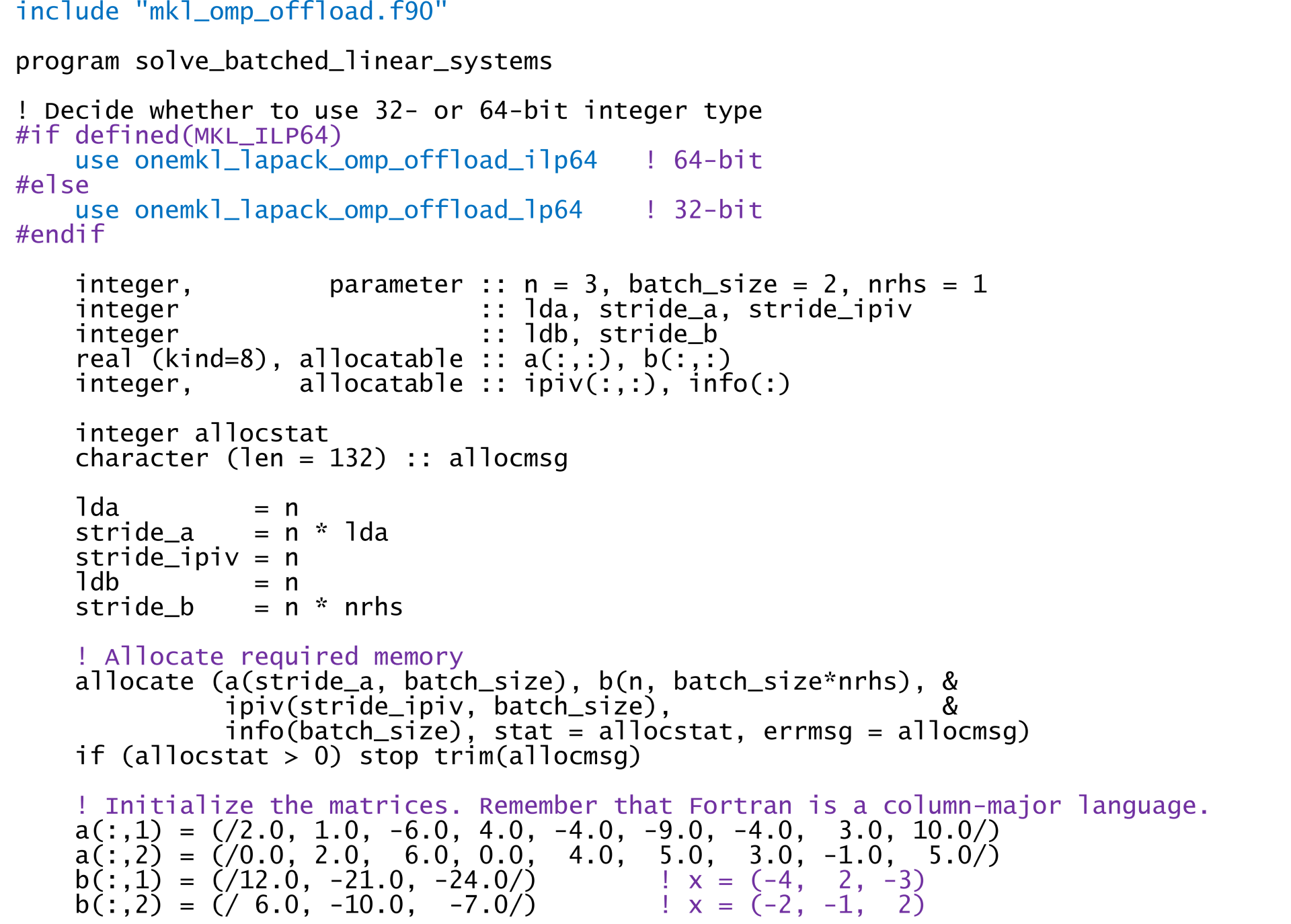
The demo program for this article is similar to the one in the previous article. It begins by including the Fortran interfaces for OpenMP offload support, then it decides whether to use 32- or 64-bit integer type (Figure 2). (See Using the ILP64 Interface vs. LP64 Interface for more information.) This decision will be made at compile-time (see the compiler command below). The test problem in Figure 1 consists of two, 3x3 linear systems, each with one right-hand side (RHS). The batch_size, n, nrhs, and stride variables are set accordingly, and the a, b, and ipiv arrays are allocated to hold the batched systems. The last four statements load the two matrices and their right-hand sides into a and b, respectively.

Figure 2. Setting up the example program. The oneMKL headers and modules that provide OpenMP* target offload support are highlighted in blue.
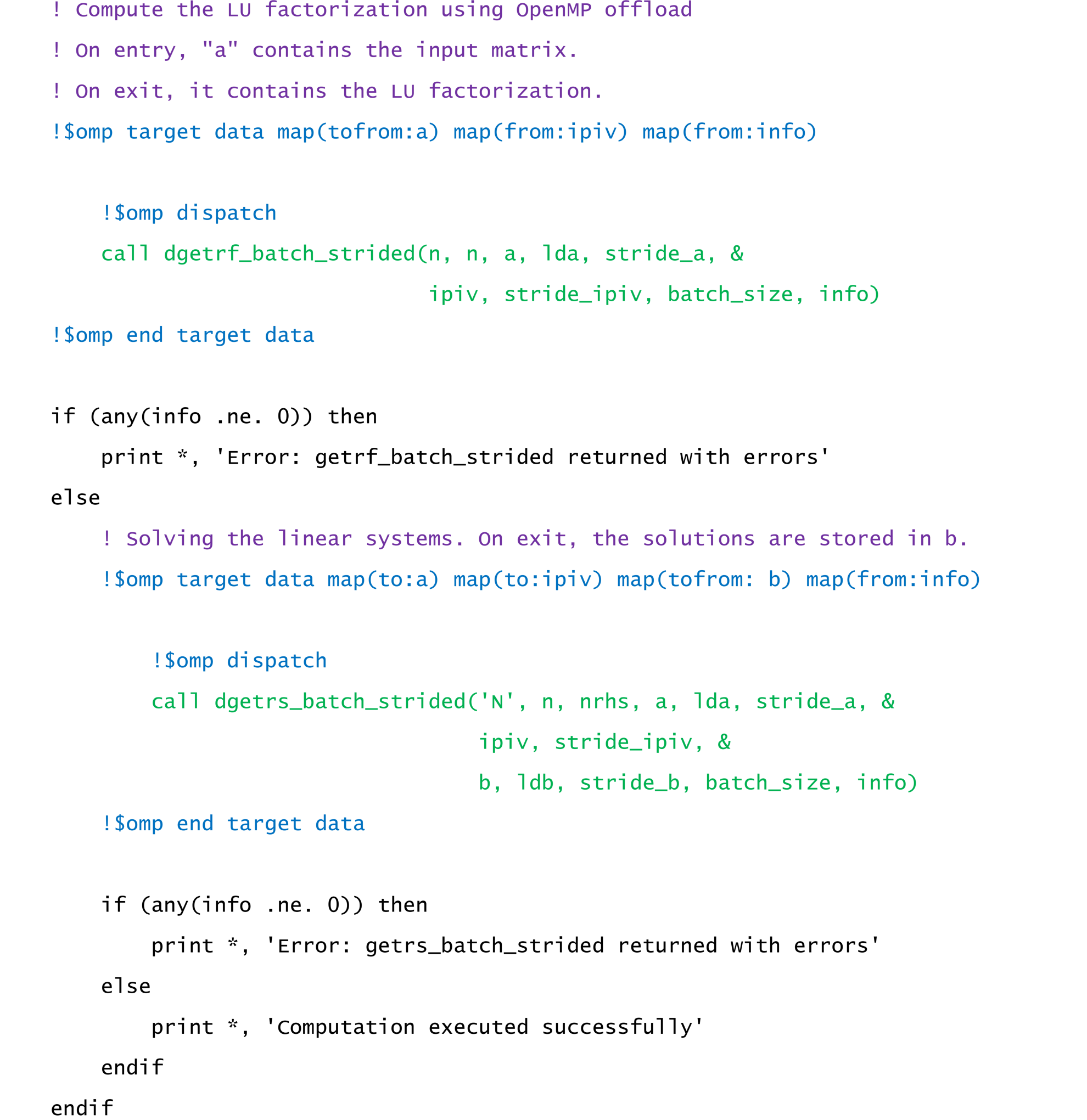
We are now ready to begin the computation. Let’s start with a basic implementation that uses two OpenMP target regions to dispatch the LU factorizations and the solutions to the linear systems (Figure 3). We compile and run the example as follows to verify that it’s giving correct results:
$ ifx -i8 -DMKL_ILP64 -qopenmp -fopenmp-targets=spir64 -fsycl -free \
> lu_solve_omp_offload_ex1_small.F90 -o lu_solve_ex1_small \
> -L${MKLROOT}/lib/intel64 -lmkl_sycl -lmkl_intel_ilp64 -lmkl_intel_thread \
> -lmkl_core -liomp5 -lpthread -ldl
$ ./lu_solve_ex1_small

=================================
 Solutions to the linear systems
=================================
   -4.0000    2.0000   -3.0000
   -2.0000   -1.0000    2.0000

Figure 3. Basic solution of batched linear systems using oneMKL and OpenMP* target offload. OpenMP directives are highlighted in blue. LAPACK calls are highlighted in green.
The target construct transfers control to the accelerator device. The first region transfers the input matrices [map(tofrom:a)] to the device memory; dispatches the in-place LU factorization (dgetrf_batch_strided) to the device; and retrieves the LU-factored matrices (now stored in a), pivot indices [map(from:ipiv)], and status [map(from:info)] from device memory. If factorization succeeded, the program proceeds to the next OpenMP region. The LU-factored matrices and pivot indices are transferred back to the device memory [map(to:a) and map(to:ipiv)] and the linear systems are solved on the device (dgetrs_batch_strided). The RHS are overwritten with the solution vectors and retrieved from the device memory [map(tofrom:b)] along with the status of the computation [map(from:info)]. The host-device data transfers are shown schematically in Figure 4.

Figure 4. Host-device data transfer for the two OpenMP* target offload regions shown in Figure 3. Each arrowhead indicates data movement between the host and device memories.
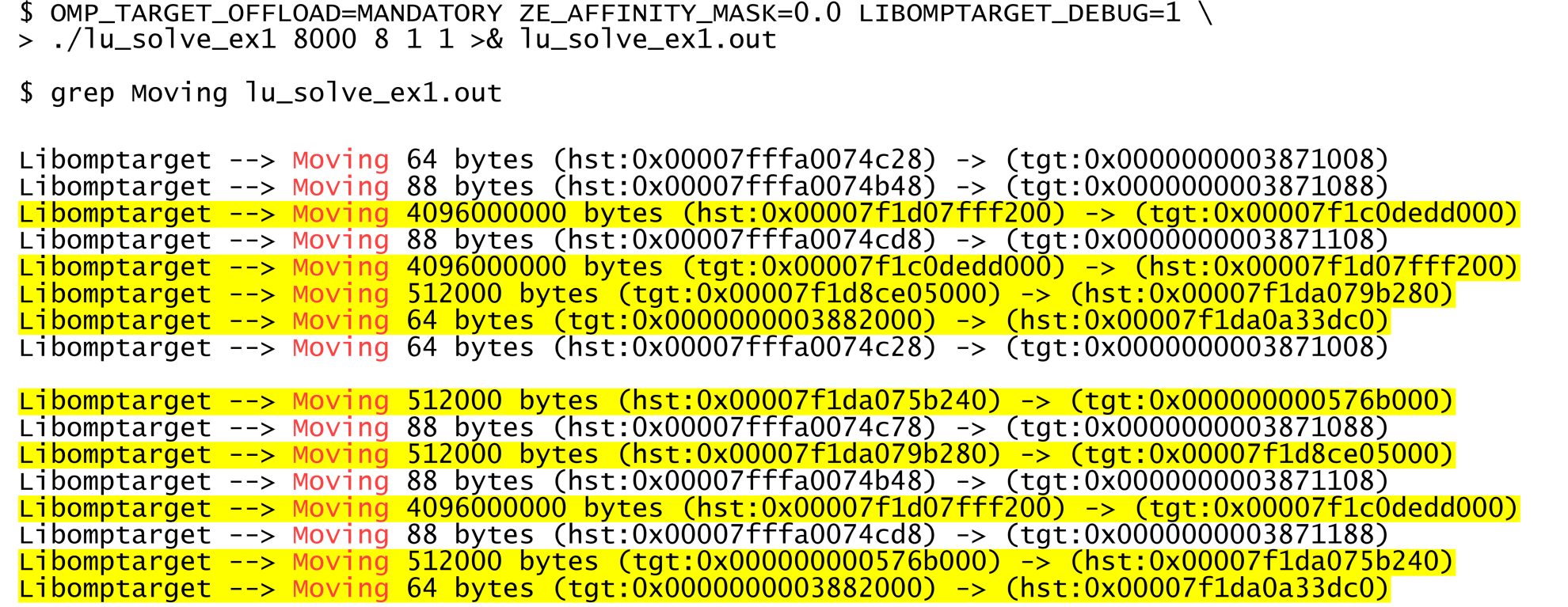
We don’t have to rely on a conceptual understanding of host-device data transfer, however. We can directly check data movement by requesting debugging information from the OpenMP runtime library, as explained in Minimizing Data Transfers and Memory Allocations. The test problem is too small to warrant acceleration, so we’ll increase the problem size to something more interesting. Let’s solve (in double precision) a batch of eight 8,000 x 8,000 linear systems, each with one RHS:

We’ve highlighted the arrays that are explicitly transferred using OpenMP map constructs and added a space to delineate the two OpenMP target regions. The unhighlighted data movements are the dope vectors of the arrays being mapped to the target device. We can ignore them because they’re generally small.
In the first target region, array a (4,096,000,000 bytes) is transferred [map(tofrom:a)] from host to target (hst→tgt) and target to host (tgt→hst). It is transferred [map(to:a)] back to the target device in the second target region. The pivots (ipiv, 512,000 bytes) are computed on the device in the first target region, retrieved [map(from:ipiv), tgt→hst], then transferred back to the device [map(to:ipiv), hst→tgt] in the second target region to compute the solutions. The RHS stored in array b (512,000 bytes) are transferred to the device, overwritten with the solution vectors, then transferred back to the host [map(tofrom:b)]. The status array, info (64 bytes), is retrieved from the device [map(from:info), tgt→hst] at the end of both target regions.
Moving data between disjoint memories takes time and energy, so we need to pay close attention to the highlighted transfers (12,290,048,128 bytes in total). With this in mind, let’s see how to improve our initial implementation.
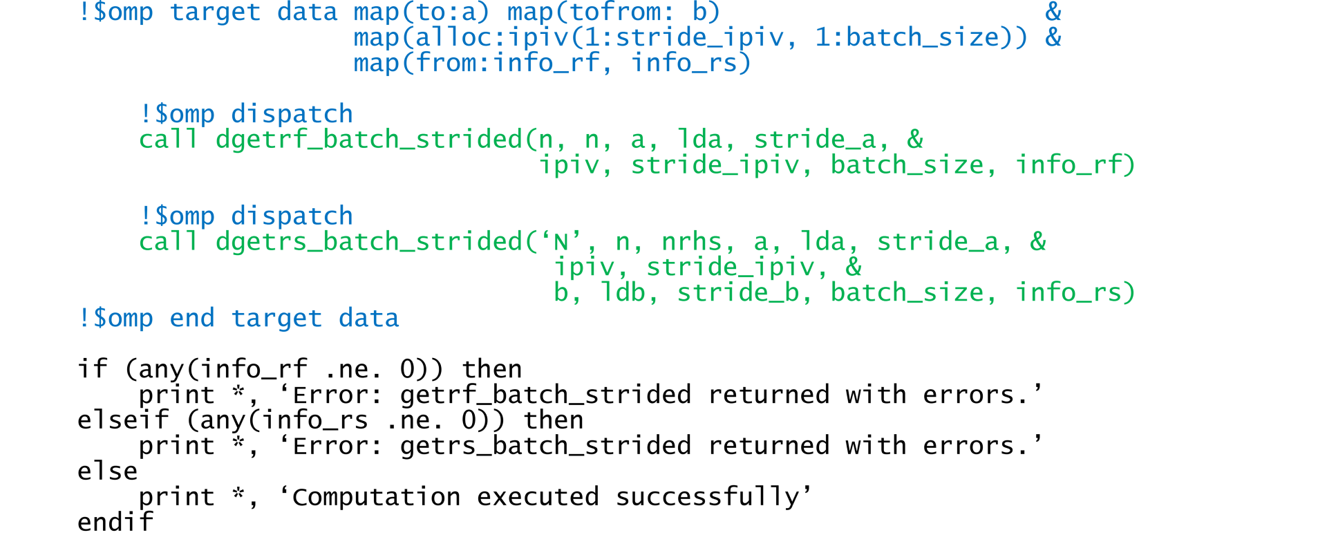
The previous article on LU factorization discussed the disadvantages of using two OpenMP target regions when one will suffice. First, transferring the control flow to the target device incurs overhead. This happens twice in the initial implementation (Figure 3). Second, redundant host-device data transfer is required (Figure 4). When solving the linear systems, we only need to copy the input arrays and RHS to the device and retrieve the solutions from the device. We also need to retrieve the status arrays, but these are relatively small. The pivots are only used by the device, so we’ll simply allocate the ipiv array directly in device memory [map(alloc:ipiv(1:stride_ipiv, 1:batch_size))]. Fusing the two OpenMP target regions results in cleaner, more concise code (Figure 5) that requires less data movement (Figure 6).

Figure 5. Using a single OpenMP* target region to solve batched linear systems with oneMKL. OpenMP directives are highlighted in blue. LAPACK calls are highlighted in green.

Figure 6. Host-device data transfer for the OpenMP* target offload region shown in Figure 5. Each arrowhead (except the one inside the accelerator device) indicates data movement between the host and device memories.
The debug information confirms this. Once again, we’ve highlighted the arrays that are explicitly transferred using OpenMP map constructs:

If we ignore the dope vectors, the single OpenMP target region in Figure 5 requires significantly less host-device data transfer (4,097,024,128 bytes) than the two target regions in the initial implementation (12,290,048,128 bytes) (Figure 3).
Minimizing host-device data transfer is a first-order concern in heterogeneous parallel computing. The code in the second example (Figure 5) significantly outperforms the original code (Figure 3), especially as the linear systems get larger (Table 1).
| Matrix Size |
CPU Time |
GPU time |
GPU time |
|---|---|---|---|
| 1,000 x 1,000 |
0.13 |
1.72 |
1.70 |
| 2,000 x 2,000 |
0.60 |
0.84 |
0.72 |
| 4,000 x 4,000 |
3.90 |
2.51 |
2.10 |
| 8,000 x 8,000 |
19.15 |
5.98 |
4.55 |
| 12,000 x 12,000 |
63.11 |
12.55 |
9.51 |
| 16,000 x 16,000 |
139.45 |
21.33 |
15.71 |
Table 1. Timing the solution of eight batched linear systems of varying matrix sizes on a Linux* (Ubuntu* 20.04 x64, 5.15.47 kernel) system with two 2.0 GHz 4th Gen Intel® Xeon® Platinum 8480+ processors (CPU), an Intel® Data Center GPU Max 1550 (GPU), and 528 GB memory. All times are in seconds. GPU tests used only one tile. Each linear system had one RHS. Each experiment was run five times. The first run was discarded because it includes the just-in-time compilation overhead for the oneMKL functions. The reported time is the sum of the remaining four runs.
The example programs used in this article are available at this repository. You can experiment with OpenMP accelerator offload on the free Intel® Developer Cloud, which has the latest Intel hardware and software.
The OpenMP target construct has many more options to give the programmer fine control over accelerator offload. We encourage you to review the OpenMP specification and example codes, and to check out the Intro to GPU Programming with the OpenMP API and Minimizing Data Transfers and Memory Allocations tutorials.
The Parallel Universe Magazine
Intel’s quarterly magazine helps you take your software development into the future with the latest tools, tips, and training to expand your expertise.