Introduction
Feature engineering1 typically refers to the process of transforming raw data to ready-to-train features. It usually requires two parts: an algorithm library to process features and a data scientist who understands the data and specifies feature engineering algorithms to enrich features and improve prediction accuracy.
Finding optimal features of data is complicated and time-consuming due to its iterative nature. To make things worse, enriching and transforming raw data on a large scale takes more time, quite often even longer than the model training stage. It was commonly reported that data scientists spent around 38% of their time on data preparation, especially feature engineering.2
To help reduce the time spent in feature engineering, we provide a workflow named Auto Feature Engineering.3 Its purpose is to simplify the feature engineering process using a built-in intelligence that maps original features or groups of features to selected engineering methods, and a powerful underlying algorithm library that keeps including more proven good methods.
The Auto Feature Engineering workflow provides an end-to-end workflow that automatically analyzes the data based on data type, profiles feature distribution, generates a customizable feature engineering pipeline, and runs the pipeline parallelly on the Intel® platform.
The workflow uses the Intel® End-to-End AI Optimization Kit4 to automatically transform raw tabular data to enriched, useful, new features on pluggable run engines such as pandas* and Apache Spark*, with the capability of integrating third-party feature engineering primitives. This can significantly improve the developer’s productivity and efficiency.
Auto Feature Engineering
Overview
The goal of the Auto Feature Engineering workflow is to shorten the time required for data scientists to process and transform large-scale raw tabular datasets to ready-to-train features. In that way, data scientists can focus more on the rest of the stages in an end-to-end (E2E) AI pipeline.
To achieve this goal, we designed an end-to-end workflow as shown in Figure 1. Figure 1 shows how data can be automatically analyzed based on data type, value distribution, and value clustering to determine which feature engineering algorithm should be applied to which feature or groups of features, resulting in a customized pipeline specially designed for this dataset. Moreover, the Auto Feature Engineering workflow provides its own feature engineering algorithm library and a pluggable interface for third-party methods. All in-house algorithms are implemented with two engines, pandas and Apache Spark, to best adapt to the user’s computing environment and provide optimal performance.

Figure 1. Auto Feature Engineering workflow architecture
The key design principle of Auto Feature Engineering is that we split the feature engineering process into multiple steps:
- Feature Profiler: Analyze a raw tabular dataset based on data type, clustering, and distribution, and then output a feature list for the Feature Engineering Pipeline generation process.
- Feature Engineering Pipeline: Use a pregenerated feature list as input, apply corresponding feature engineering algorithms to each feature, and generate a data pipeline as output. This data pipeline can be exported in json/yaml file format for the user to view, modify, and reload.
- Feature Transformation: Use the data pipeline and original data as input, based on a user-selected compute engine, convert the data pipeline to executable codes, and then do the execution to transform original data to ready-to-train features.
Feature Importance Estimation: Use transformed ready-to-train features as input and perform feature importance analysis to get the feature importance rank, which can be used for the user to understand the effectiveness of each feature.
How it Works
The default API to run Auto Feature Engineering on your dataset requires only three lines of codes.
from pyrecdp.autofe import AutoFE

pipeline = AutoFE(dataset=train_data, label=target_label, time_series = 'Day')
transformed_train_df = pipeline.fit_transform()
Figure 2. Auto Feature Engineering workflow to generate a pipeline and transform data to ready-to-train enriched features
The only thing a data scientist needs to do is to prepare a pandas dataframe and provide it to the Auto Feature Engineering component (the AutoFE module in Figure 2). AutoFE module will create a pipeline based on the provided data and target label, and then run the pipeline with fit_transform() API to get enriched features.
Figures 3 and Figure 4 provide a preview of the raw and processed data to highlight the transformation.
In Figure 3 there are 14 columns in the original dataset. The feature ‘Is Fraud?’ is the target label and the remaining 13 features are regarded as original features.
In Figure 4, after Auto Feature Engineering transformation, there are 55 columns in the dataset. Auto Feature Engineering automatically standardizes column names (including features name or target label name), thus the target label ‘Is Fraud?’ is renamed to ‘Is_Fraud’. The remaining 54 features are ready-to-train, of which 40 features are created by Auto Feature Engineering.

Figure 3. Raw data (with 13 original features and 1 target label)

Figure 4. Transformed data after Auto Feature Engineering (with 54 original features and 1 target label)
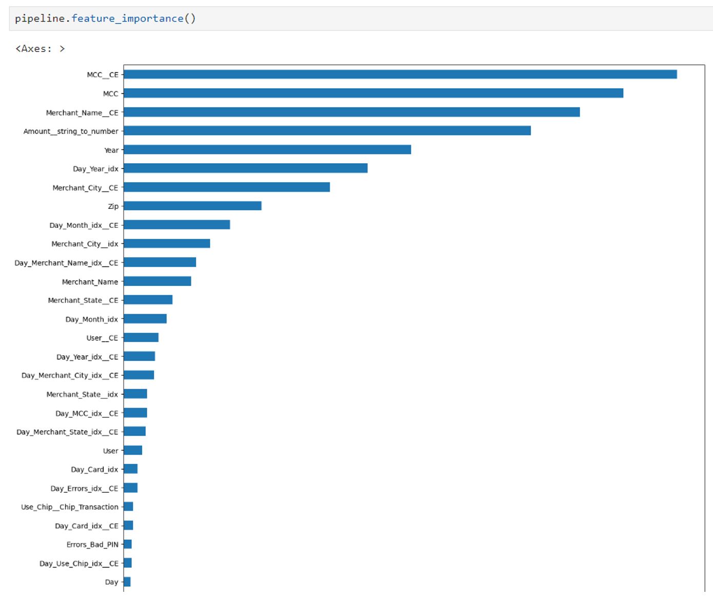
Auto Feature Engineering also provides an API to view the feature importance of enriched datasets. For example, as shown in Figure 5, feature names with ‘*__CE’, ‘*__idx’, and ‘Day_*’ are created by Auto Feature Engineering through count encoding, categorify, and time_series algorithms. Features such as ‘Use_chip__Chip_Transaction’, and ‘Use_chip__online_Transaction’, are created by Auto Feature Engineering through encoding.

Figure 5. Feature importance list (new features created by AutoFE show high importance)
To process the test and validation dataset, we need to transform them with the same pipeline applied to the training dataset as shown in Figure 6.
from pyrecdp.autofe import AutoFE

pipeline = AutoFE(dataset=train_data, label=target_label, time_series = 'Day')
transformed_train_df = pipeline.fit_transform()

valid_pipeline = AutoFE.clone_pipeline(pipeline, valid_data)
transformed_valid_df = valid_pipeline.transform()

test_pipeline = AutoFE.clone_pipeline(pipeline, test_data)
transformed_test_df = test_pipeline.transform()
Figure 6. Generate the pipeline from the training dataset and apply it to the test and validation dataset.
Now we have transformed the train, validation, and test dataset, which can fit models such as LightGBM or XGBoost. The performance section gives more information about the accuracy improvement on multiple different datasets.
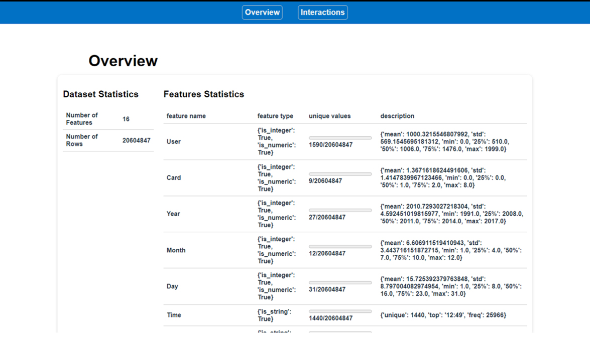
Auto Feature Engineering component provides additional APIs for customization, which enable the user to view data profiling, data pipeline, customize the pipeline, save, and reload the pipeline for future usage.
View Data Profiling
pipeline.profile()

Figure 7. Example screenshot for feature profiling
View Data Pipeline
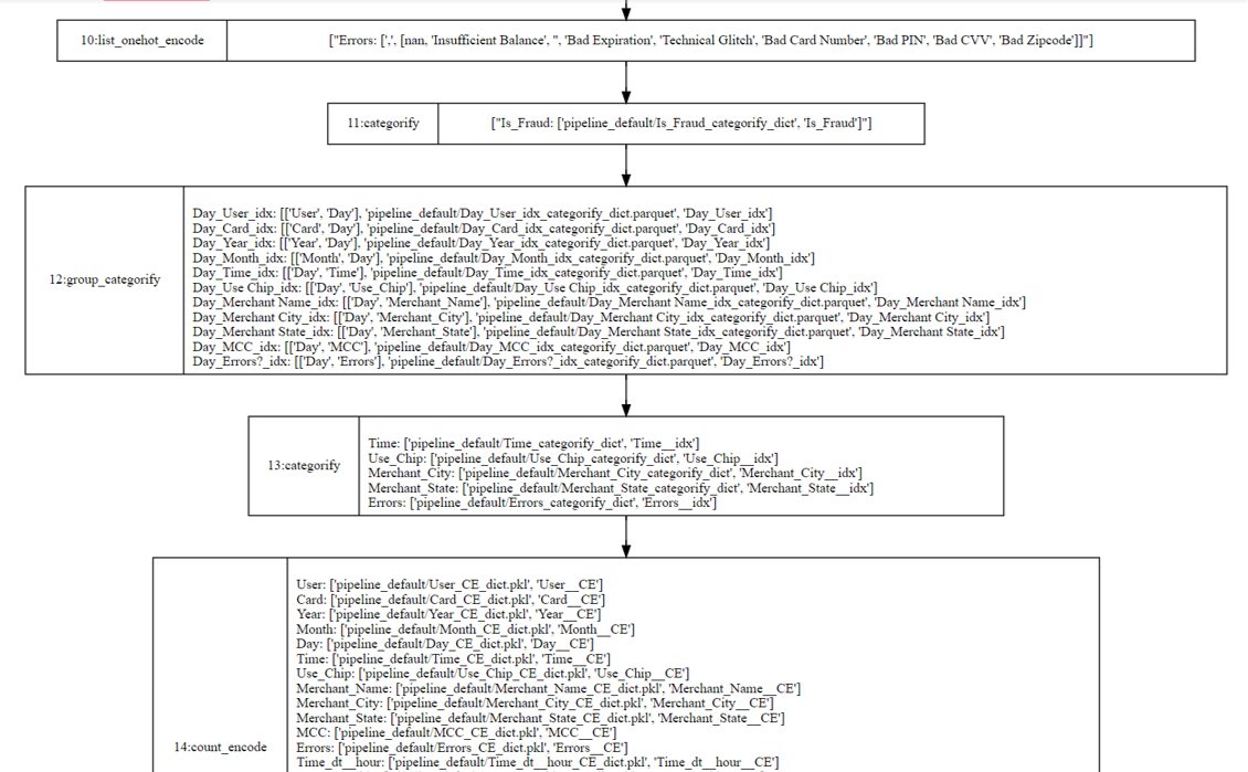
pipeline.plot()

Figure 8. Example screenshot for data pipeline (For a completed version, see the Auto Feature Engineering Data Pipeline Example13)
Customize with Your Own Dataset Data Pipeline
Define your own function and plug it into the Auto Feature Engineering pipeline, which enriches the transformed data with your own function.
def process_feature_with_condition(df):
    df.loc[df['year'] <= 2018, 'early_year'] = 'True'
    df.loc[df['year'] > 2018, 'early_year'] = 'False'
    return df
Figure 9. Example screenshot for customized function (input and output should be a pandas data frame)
from pyrecdp.autofe import AutoFE

pipeline = AutoFE(dataset=train_data, label=target_label)
# Add customized function
pipeline.add_operation(process_feature_with_condition)
transformed_train_df = pipeline.fit_transform()
Figure 10. Example screenshot to plug in a customized function into the Auto Feature Engineering pipeline
Performance
Testing Methodology
To showcase the performance, we compare Auto Feature Engineering (AutoFE) with other two automatic feature engineering tools: Featuretools5 and AutoGluon6. Three different datasets are selected to show the performance in two dimensions: productivity and speed. Line of codes (LOC) serves as the metric to evaluate productivity, and higher LOC means the user needs to write more codes to use the toolkit. Time serves as the metric of speed. We use the time (in seconds) needed to generate new features and normalize to seconds/feature as the generated feature numbers vary for different tools.
To evaluate the performance, we use different metrics for each use case.
- For NYC taxi fare prediction7, which is used to predict linear fare for each trip, we use Root Mean Square Error (RMSE) to evaluate the result and a lower value indicates better prediction.
- For Fraud Detection classification8, which is used to classify if one event is fraud or not, we use Area Under the Precision-Recall Curve (AUCPR) to evaluate, and a higher value indicates better classification.
- For Recsys2023 classification9, which is used to classify if one application is installed or not. We use Area Under Curve (AUC) to evaluate, and a higher value indicates better classification.
Performance Result
Overall, Auto Feature Engineering shows better performance in both productivity and speed for all three use cases. As shown in Figure 11, the Y-axis indicates the line of codes (LOC) (lower is better), the X-axis indicates the processing time(seconds) (lower is better), and the bubble size indicates the normalized accuracy (higher is better).
The diagram is divided into four quadrants, and we use 50 lines of code and 30 minutes of processing time as partition factors.

Figure 11. Performance overview for Auto Feature Engineering (AutoFE), Featuretools and AutoGluon
For the Recsys2023 dataset, which contains 3 million lines of records, Auto Feature Engineering improves AUC by 1.08x and 1.02x to AutoGluon and Featuretools respectively.12 All three tools took less than 30 minutes to complete the data preparation.
For the Fraud Detect dataset, which contains 24 million lines of records, AUCPR is 2.5% lower than Featuretools and 1.08x better than AutoGluon.10 All three tools took less than 30 minutes to complete the data preparation.
For NYC Taxi Fare dataset, which contains 55 million lines of records, Auto Feature Engineering improves RMSE by 1.02x and 1.19x to AutoGluon and Featuretools respectively.11 Featuretools and AutoGluon take more than 30 minutes for feature engineering, and the Auto Feature Engineering workflow took around 250 seconds to complete data preparation with an optimal RMSE score. Also, to provide equivalent accuracy for the NYC Taxi Fare dataset, Featuretools requires around 70 lines of codes to provide the functionality, and AutoGluon and Auto Feature Engineering only takes 3 lines of code.
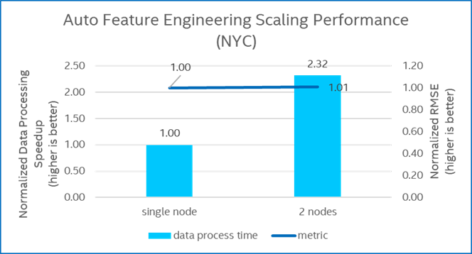
Figure 12 provides the scaling performance to run Auto Feature Engineering on NYC Taxi Fare dataset with two nodes. Compared to running with single node, the processing speedup is around 2.32x, which is improved by nodes scaling from 1 to 2 and switching from Apache Spark local mode to stand-alone mode.

Figure 12. Auto Feature Engineering Scaling Performance
Conclusion
In this blog, we demonstrate the productivity and speed benefit of using the Auto Feature Engineering workflow to enrich raw data. It is extremely easy to deploy and takes only three lines of code to adapt to any tabular dataset and customize with your own domain-specific functions. For more details, see the Auto Feature Engineering workflow on GitHub*.
Additional Resources
Check out Intel’s other AI Tools and Framework optimizations.
Learn about the unified, open, standards-based oneAPI programming model that forms the foundation of Intel’s AI Software Portfolio.
References
- Wikipedia - Feature Engineering
- Anaconda Report - State of Data Science Survey
- Auto Feature Engineering workflow on GitHub*
- GitHub - Intel® End-to-End AI Optimization Kit
- Documentation - Featuretools
- Documentation - AutoGluon
- Kaggle Competition - New York City Taxi Fare Prediction
- GitHub - Tabular Transformers for Modeling Multivariate Time Series
- RecSys Challenge 2023
- FraudDetect Use Case Notebook
- NYC Taxi Fare Use Case Notebook
- Recsys2023 Use Case Notebook
- Auto Feature Engineering Data Pipeline Example
- Creating an AI-Based Customer Segmentation Model Using Intel-Optimized Workflows
- Act-On Software collaborates with Intel to Accelerate AI Audience Insights to Market
- Enhanced Fraud Detection Using Graph Neural Networks with Intel Optimizations
- Document Automation Reference Use Case: End-to-End AI Augmented Semantic Search System
System Configurations
The tests were conducted on a single-node cluster and a two-node cluster. Each node is equipped with Intel® Xeon® Platinum 8352Y CPU @ 2.20 GHz and 512 GB memory. Configuration details are shown in the following table. Test by Intel in July 2023.
Table 1. Hardware configuration for the experiment
| Name | Description |
|---|---|
| CPU |
Intel® Xeon® Platinum 8352Y CPU @ 2.20GHz |
| Memory Size |
>100 GB |
| Disk Size |
>300 GB |
| Number on nodes |
1 or 2 nodes |
Table 2. Software configuration for the experiment
|
Package |
Version |
|---|---|
|
OS |
Ubuntu 22.04 |
|
Docker compose |
2.7.x or later |
|
Python |
3.8.10 |
|
Apache Spark |
3.4.1 |
|
Pandas |
2.0.1 |
|
Featuretools |
1.26.0 |
|
AutoGluon |
0.8.2 |
|
LighGBM |
3.3.5 |
|
XGBoost |
1.7.5 |
