Contributors:
Xu, Qing
Liu, Shengxian
Ma, Hua
Du, Jessica
Lei, Ming
Wang, Yang
Introduction
In this document, we introduce how to optimize the PointPillars [3], a network for the DL-based object detection in 3D point clouds, on the 11th-Generation Intel® Core™ Processors (Tiger Lake) by using the Intel® Distribution of OpenVINO™ Toolkit.
The throughput requirment for the use cases of transportation infrastructure (e.g., 3D point clouds generated by the roadside Lidars) is 10 FPS. In comparison with the existing solutions that we are aware of, our solution can achieve the throughput of 11.1 FPS and the latency of 154.7 ms on Intel® Core™ processors.
Key words:
Intel Core Processor, Tiger Lake, CPU, iGPU, OpenVINO, PointPillars, 3D Point Cloud, Lidar, Artificial Intelligence, Deep Learning, Intelligent Transportation.
PointPillars
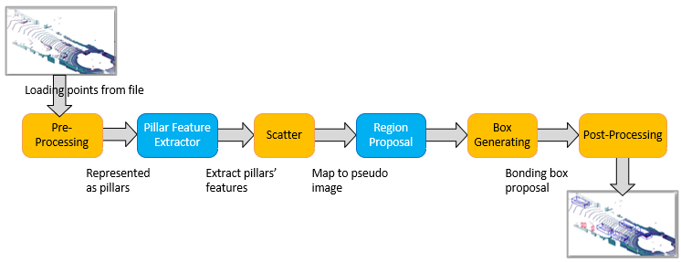
The PointPillars [1] is a fast E2E DL network for object detection in 3D point clouds. It utilizes PointNets to learn a representation of point clouds organized in vertical columns (pillars). Extensive experimentation shows that PointPillars outperforms previous methods with respect to both speed and accuracy by a large margin [1].

The above figure shows the main steps (components) of the PointPillars network:
- PFN
- Pre-processing: It converts raw data of point clouds to a stacked pillar tensor and pillar index tensor;
- PFE: It uses the stacked pillars to learn a set of features;
- Scattering: It scatters the pillar features back to a 2D pseudo-image for a CNN.
- Backbone (2D CNN)
- RPN: It utilizes CNN to extract the features from a 2D pseudo-image.
- Detection Head (SSD)
- Prediction of 3D Bounding Boxes: the features from the Backbone are used by the Detection Head to predict 3D bounding boxes for objects;
- Post-Processing: to filter the boxes with NMS algorithm.
OpenVINO™ Toolkit
It is a comprehensive toolkit for quickly developing applications and solutions that solve a variety of tasks including emulation of human vision, automatic speech recognition, natural language processing, recommendation systems, and many others.
Based on latest generations of artificial NNs, including CNNs, recurrent and attention-based networks, the toolkit extends computer vision and non-vision workloads across Intel® hardware, maximizing performance. It accelerates applications with high-performance, AI and DL inference deployed from edge to cloud.
The release (version) of OpenVINO™ toolkit used in this work is 2021.3
11th-Gen Intel® Core™ Processors (Tiger Lake)
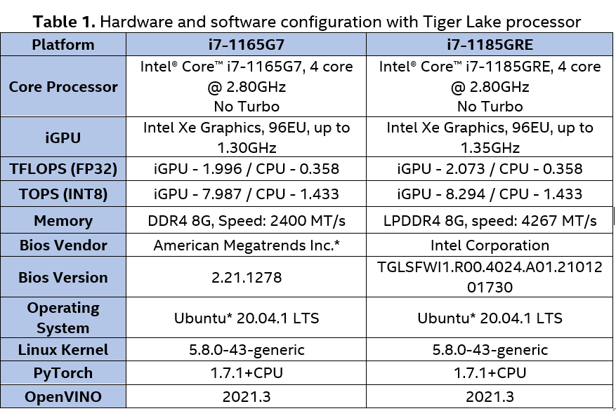
Two SKUs of the 11th-Gen Intel® Core™ processors (Tiger Lake) are used in this work:
- Intel® Core™ i7-1185GRE processor (detailed specs in [3])
- Intel® Core™ i7-1165G7 processor (detailed specs in [4])
All our test results presented in this document, are collected from below 2 platforms:
Performance Evaluation Results
With the optimization methods described in the following sections, we can achieve the throughput of 11.1 FPS and the latency of 154.7 ms on Intel® Core™ i7-1185GRE processor (with the Turbo mode disabled).
The performance evaluation results on different hardware platforms are shown in Table 2.
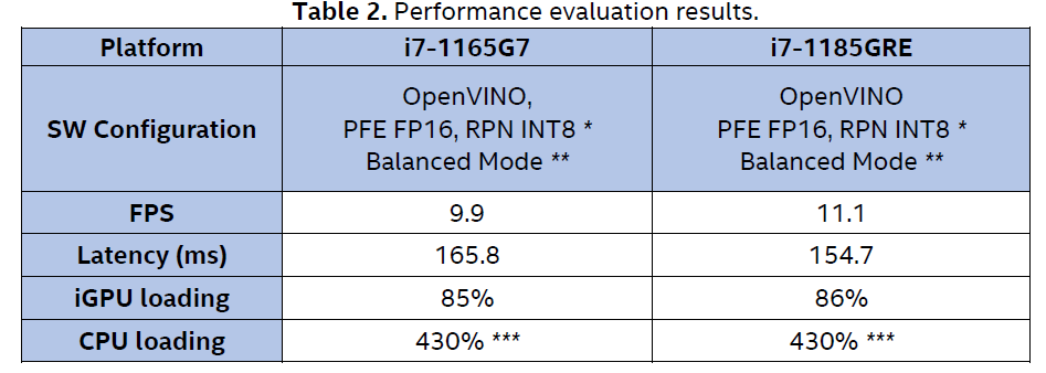
PFE FP16, RPN INT8* - Refer to Section "Quantization to INT8"
Balanced Mode** - Refer to Section "Balanced Mode"
430%*** - We get cpu loading by ‘top’ tool on Ubuntu*20.04. ‘top’ displays cpu loading as a percentage of a single CPU. On multi-core systems, you can have percentages that are greater than 100%. In Intel® Core™ i7-1165G7 or Intel® Core™ i7-1185GRE, there are 4 physical cores with 2 threads for each core, so, there are 8 logical cores in total, therefore, the highest loading would be 8x100% = 800%.
Migration of Source Codes
We leverage the open-source project OpenPCDet [5], which is a sub-project of OpenMMLab [6]. OpenPCDet framework supports several models for object detection in 3D point clouds (e.g., the point cloud generated by Lidar), including PointPillars.
The original OpenPCDet is implemented by official released PyTorch* (we verified on PyTorch 1.7.1+CPU). And, in PointPillars pipeline, it contains the following components:
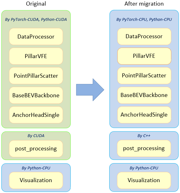
The original source codes cannot run on Intel® architecture as they are developed in the CUDA environment. Therefore, in order to support the OpenPCDet on general-purpose CPUs without the CUDA environment, we perform the migration of the source codes which are described in the following sections.
Migration of PyTorch* Source Codes
As shown in the following examples, the ".cuda()" appear in the original source codes. They need to be removed in the migration.
- model.cuda()
+   device = 'cpu'
+   model.to(device)
-   self.anchors = [x.cuda() for x in anchors]
+   self.anchors = [x for x in anchors]
-   batch_dict[key] = torch.from_numpy(val).float().cuda()
+   batch_dict[key] = torch.from_numpy(val).float()
Migration to C++ Source Codes
CUDA kernels in the original source codes need to be replaced by the standard C++.
CUDA compiler is replaced by C++ compiler.
-  from torch.utils.cpp_extension import BuildExtension, CUDAExtension
+  from torch.utils.cpp_extension import BuildExtension, CppExtension
CUDA source codes are removed from the compiling configuration file.
                 sources=[
                     'src/pointnet2_api.cpp',
                     'src/ball_query.cpp',
-                    'src/ball_query_gpu.cu',
                     'src/group_points.cpp',
-                    'src/group_points_gpu.cu',
                     'src/sampling.cpp',
-                    'src/sampling_gpu.cu',
                     'src/interpolate.cpp',
-                    'src/interpolate_gpu.cu',
                   ],
Calls to CUDA kernels are removed.
- nmsLauncher(boxes_data, mask_data, boxes_num, nms_overlap_thresh);
- nmsNormalLauncher(boxes_data, mask_data, boxes_num, nms_overlap_thresh);
In the PointPillars, only the NMS algorithm is implemented as CUDA kernel. We just need to re-write it manually with C++.
+void nmsLauncher(const float *boxes, bool *mask,
+                 const int boxes_num, const float nms_overlap_thresh){
+     int col_idx = 0;
+     int row_idx = 0;+
+     float block_boxes[7];
+     mask[0] = false;
+     for (col_idx = 0; col_idx < boxes_num; col_idx++){
+         if (mask[col_idx]==true)
+         continue;
+     block_boxes[0] = boxes[col_idx * 7 + 0];
+     block_boxes[1] = boxes[col_idx * 7 + 1];
+     block_boxes[2] = boxes[col_idx * 7 + 2];
+     block_boxes[3] = boxes[col_idx * 7 + 3];
+     block_boxes[4] = boxes[col_idx * 7 + 4];
+     block_boxes[5] = boxes[col_idx * 7 + 5];
+     block_boxes[6] = boxes[col_idx * 7 + 6];
+
+     for (row_idx = col_idx + 1; row_idx < boxes_num; row_idx++){
+         const float *cur_box = boxes + row_idx * 7;
+         bool drop = 0;
+
+         if (iou_bev(cur_box, block_boxes) > nms_overlap_thresh){
+            drop = true;
+            mask[row_idx] = drop;
+         }
+      }
+   }
+}
Profiling on Intel® Core™ Processors (Tiger Lake)
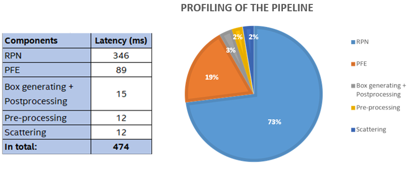
After the migration of source codes, we run and collect the performance data of the PointPillars network on the Intel® Core™ i7-1165G7 processor, the hardware and software configuration as shown in Table 2.
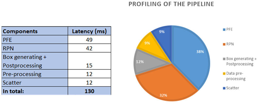
As shown in Figure 3, the two NN models (RPN and PFE) are the the most time-consuming components, accounting for 92% of the total latency. Therefore, we need to focus on the optimizaiton of these models.
Implementation with OpenVINO™ Toolkit
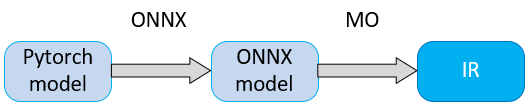
As a part of the OpenVINO™ toolkit, the MO is a cross-platform command-line tool that facilitates the transition between the training and deployment environment, performs static model analysis, and adjusts NN models for optimal execution on end-point target devices. Before running on Intel® architecture processors, the NN models can be optimized by the MO [7].
The MO converts the NN model to the IR format, which can be read, loaded, and inferred with the IE. IE offers a unified API across a number of supported Intel® architecture processors. The IR format uses a pair of files to describe the NN model:
- .xml file describing the topology of the NN;
- .bin file containing the binary data for the weights and biases.

Conversion of NN Models to IR
In this section, we will show how to convert the NN models used in PointPillars from the PyTorch* to the IR format, and to integrate them into the processing pipeline.
As MO does not support the direct conversion from the PyTorch* to the IR format, we need to convert the models from the PyTorch* to the ONNX format as an intermediate step (as shown in Figure 5).
ONNX [8] is an open ecosystem that empowers AI developers to choose the right tools as their project evolves. ONNX provides an open source format for AI models, both DL and traditional ML. It defines an extensible computation graph model, as well as definitions of built-in operators and standard data types.
As mentioned in Section3.1, there are two NN models used in PointPillars [1]: PFE and RPN. We need to convert them to the IR format.
Conversion from PyTorch* to ONNX
We leverage the open-source project SmallMunich [9], to convert the NN models from PyTorch* to ONNX, by following instructions in https://github.com/SmallMunich/nutonomy_pointpillars#onnx-ir-generate.
SmallMunich is also Pytorch*-based codebase for PointPillars. Additionally, it implements ONNX conversion. By running onnx_model_generate(), we get the ONNX models (pfe.onnx and rpn.onnx) from the PyTorch* models.
Conversion from ONNX to IR
Run the MO to convert pfe.onnx to the IR format (FP16):
$ cd <install_folder>/openvino_2021/deployment_tools/model_optimizer

$ python mo.py --input_model <input_folder>/pfe.onnx --input pillar_x,pillar_y,pillar_z,pillar_i,num_points_per_pillar,x_sub_shaped,y_sub_shaped,mask --

input_shape=[1,1,12000,100],[1,1,12000,100],[1,1,12000,100],[1,1,12000,100],[1,12000],[1,1,12000,100],[1,1,12000,100],[1,1,12000,100] -o <output_folder> --data_type=FP16
Output is as follows:
Model Optimizer arguments:
Common parameters:

                  - Path to the Input Model: <your_input_folder>/pfe.onnx
                  - Path for generated IR: <your_output_folder>
                  - IR output name: pfe
                  - Log level: ERROR
                  - Batch: Not specified, inherited from the model
                  - Input layers: pillar_x,pillar_y,pillar_z,pillar_i,num_points_per_pillar,x_sub_shaped,y_sub_shaped,mask
                  - Output layers: Not specified, inherited from the model
                  - Input shapes: [1,1,12000,100],[1,1,12000,100],[1,1,12000,100],[1,1,12000,100],[1,12000],[1,1,12000,100],[1,1,12000,100],[1,1,12000,100]
                  - Mean values: Not specified
                  - Scale values: Not specified
                  - Scale factor: Not specified
                  - Precision of IR: FP16
                  - Enable fusing: True
                  - Enable grouped convolutions fusing: True
                  - Move mean values to preprocess section: None
                  - Reverse input channels: False
ONNX specific parameters:
                  - Inference Engine found in: <install_folder>/openvino_2021/python/python3.8/openvino
Inference Engine version: 2.1.2021.3.0-2787-60059f2c755-releases/2021/3
Model Optimizer version: 2021.3.0-2787-60059f2c755-releases/2021/3
[ SUCCESS ] Generated IR version 10 model.
[ SUCCESS ] XML file: <your_output_folder>/pfe.xml
[ SUCCESS ] BIN file: <your_output_folder>/pfe.bin
[ SUCCESS ] Total execution time: 3.67 seconds.
[ SUCCESS ] Memory consumed: 281 MB.
Run the MO to convert rpn.onnx to the IR format (FP16):
$ cd <install_folder>/openvino_2021/deployment_tools/model_optimizer
$ python mo.py --input_model <input_folder>/rpn.onnx -o <output_folder> --input_shape=[1,64,496,432] --data_type=FP16
Output is as follows:
Model Optimizer arguments:
Common parameters:
           - Path to the Input Model: <your_intput_folder>/rpn.onnx
           - Path for generated IR: <your_output_folder>
           - IR output name: rpn
           - Log level: ERROR
           - Batch: Not specified, inherited from the model
           - Input layers: Not specified, inherited from the model
           - Output layers: Not specified, inherited from the model
           - Input shapes: [1,64,496,432]
           - Mean values: Not specified
           - Scale values: Not specified
           - Scale factor: Not specified
           - Precision of IR: FP16
           - Enable fusing: True
           - Enable grouped convolutions fusing: True
           - Move mean values to preprocess section: None
           - Reverse input channels: False
ONNX specific parameters:
           - Inference Engine found in: <install_folder>/openvino_2021/python/python3.8/openvino
Inference Engine version: 2.1.2021.3.0-2787-60059f2c755-releases/2021/3
Model Optimizer version: 2021.3.0-2787-60059f2c755-releases/2021/3
[ SUCCESS ] Generated IR version 10 model.
[ SUCCESS ] XML file: <your_output_folder>/rpn.xml
[ SUCCESS ] BIN file: <your_output_folder>/rpn.bin
[ SUCCESS ] Total execution time: 7.25 seconds.
[ SUCCESS ] Memory consumed: 384 MB.
Finally, we get the IR format files as the output of MO, for the two NN models used in PointPillars.
- PFE model: pfe.xml and pfe.bin;
- RPN model: rpn.xml and rpn.bin.
Verification with Benchmark Tool
We use Benchmark Tool to evaluate the throughput (in FPS) and latency (in ms) by running each NN model. The evaluation results provides the guidance for further optimization.
Benchmark Tool is a software provided by the OpenVINO™ toolkit. It creates the simulated inputs to evaluate the NN model’s performance. This software supports two operating modes: "sync" and "async" (default mode).
We evaluate the throughput and latency of CPU and iGPU in Intel® Core™ i7-1165G7 processor by using the following commands:
$ cd ~/intel/openvino_2021/deployment_tools/tools/benchmark_tool/

$ python3 benchmark_app.py -m <folder>/pfe.xml -d CPU -api sync
$ python3 benchmark_app.py -m <folder>/rpn.xml -d CPU -api sync

$ python3 benchmark_app.py -m <folder>/pfe.xml -d GPU -api sync
$ python3 benchmark_app.py -m <folder>/rpn.xml -d GPU -api sync
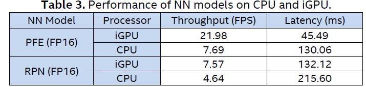
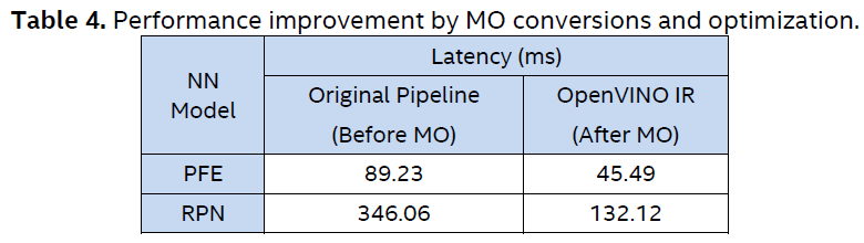
From the evaluation results shown in Table 3 and Table 4, we observed that:
- iGPU outperforms CPU in throughput and latency for both NN models;
- The processing of NN models (in IR format) converted and optimized by the MO can be significantly accelerated.
Quantization to INT8
To further accelerate the inference, we use the POT [10] to convert the RPN model from the FP16 to the INT8 resolution (while the work on PFE model is still in progress).
The POT is designed to accelerate the inference of NN models by a special process (example, post-training quantization) without retraining or fine-tuning the NN model. Therefore, there is no need for additional training datasets or further processing.
The sample codes for the POT can be found in the OpenVINO™ toolkit:
<install_folder>/openvino_2021/deployment_tools/tools/post_training_optimization_toolkit/sample
Annex A shows the Python* scripts used in our work.
In the following scripts, we choose the algorithm 'DefaultQuantization' (without accuracy checker), and the preset parameter 'performance' (the symmetric quantization of weights and activations).
algorithms = [
   {
      'name': 'DefaultQuantization',
      'params': {
          'target_device': 'CPU',
          'preset': 'performance',
          'stat_subset_size': 100
                }
   }
]
In the following scripts, the _getitem_() is the most important function and it is called by the POT to process the input dataset.
The img is the input dataset. We get the input of RPN model from the SmallMunich evaluation pipeline (the input is a matrix of [1, 64, 496, 432]).
The annotation is used by the accuracy checker to verify whether the predicted result is same as annotation. However, as we choose the algorithm 'DefaultQuantization', the accuracy checker skips the comparison. Therefore, we just need to provide an annotation of all zeros with exactly the same shape of the output of the RPN inference.
def __getitem__(self, index):
    ...
    img = np.fromfile(image_path, dtype=np.float32).reshape(64,496,432)
    annotation_np = {'184': np.zeros((1, 248, 216, 14), dtype=np.float32),
                     '185': np.zeros((1,248,216,2), dtype=np.float32),
                     '187': np.zeros((1,248,216,4), dtype=np.float32)}
    annotation = (index, annotation_np)
    return annotation, img
After running the following POT scripts, we will have the RPN model in IR format (rpn.xml and rpn.bin) with INT8 resolution.
INFO:compression.statistics.collector:Start computing statistics for algorithms : DefaultQuantization
INFO:compression.statistics.collector:Computing statistics finished
INFO:compression.pipeline.pipeline:Start algorithm: DefaultQuantization
INFO:compression.algorithms.quantization.default.algorithm:Start computing statistics for algorithm : ActivationChannelAlignment
INFO:compression.algorithms.quantization.default.algorithm:Computing statistics finished
INFO:compression.algorithms.quantization.default.algorithm:Start computing statistics for algorithms : MinMaxQuantization,FastBiasCorrection
INFO:compression.algorithms.quantization.default.algorithm:Computing statistics finished
INFO:compression.pipeline.pipeline:Finished: DefaultQuantization
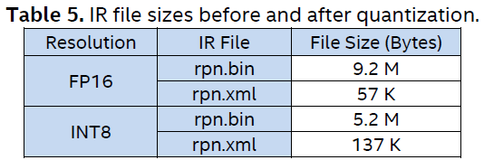
Table 5 shows that the quantization can significantly reduce the file size for the RPN model weights from 9.2 MB (FP16) to 5.2 MB (INT8).
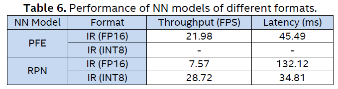
Using the Benchmark Tool, we evaluated the two NN models of different formats and resolutions on the CPU and iGPU in Intel® Core™ i7-1165G7 processor and the performance results are shown in Table 6. Given the benchmark results and the fact that the quantization of the PFE model is still in progress, we decided to use the PFE (FP16) and RPN (INT8) models in the processing pipeline for the PointPillars network.
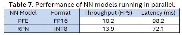
We also run the Benchmark Tool for the PFE (FP16) and RPN (INT8) models in parallel on the iGPU in Intel® Core™ i7-1165G7 processor. The results shown in Table 7 can give us some guidance on parallelizing the pipeline.
Integration of IE into PointPillars Pipeline
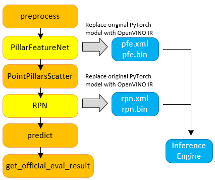
As shown Figure 7, we integrate the IR files of two NN models into the SmallMunich pipeline.
- PFE model: pfe.xml and pfe.bin;
- RPN model: rpn.xml and rpn.bin.
Besides the C++ API, the OpenVINO™ toolkit also provides the Python* API to call the IE.
The integration of the IE into the PointPillars pipeline includes the following steps shown in Figure 8.

- Create IE Core to manage available devices and read network objects;
- Read the NN model of IR format created by the MO (.xml is the supported format);
- Configure input and output;
- Load the NN model to the device;
- Create an inference request;
- Prepare the input;
- Inference;
- Process the output.
Initialization of IE
We create the IE core instance to handle both PFE and RPN inferences.
ie = IECore()
Loading NN Model and Inference
The main idea in integration, is to replace the forward() function of PyTorch* with the infer() function (Python* API) of OpenVINO™ toolkit.
PFE Model
First, read network’s topology and weights to memory.
model_file_pfe = "<your_folder>/pfe.xml"
model_weight_pfe = "<your_folder>/pfe.bin"
net = openvino_ie.read_network(model_file_pfe, model_weight_pfe)
Then, we need to tell IE information of input blob and load network to device.
For the PFE model, it's input shape is variable for each point cloud frame, as the number of pillars in each frame varies. Therefore, there are two methods of shaping the input: Static Input Shape and Dynamic Input Shape. The former method is used in our work.
- Static Input Shape
Call load_network() to load the model to GPU. In pfe.xml file, it has defined the input shape as [[1,1,12000,100], [1,1,12000,100], [1,1,12000,100],[1,1,12000,100],[1,12000],[1,1,12000,100], [1,1,12000,100], [1,1,12000,100]]
exec_net = openvino_ie.load_network(network=self.net_pfe, device_name="GPU")
Then, we utilize zero padding to set the input blob’s shape to 12000. According to it's original configuration in the source code, which means we expect maximum to 12000 pillars as the input to the network.
len_padding = 12000 - pillar_len
pillarx_pad = np.pad(pillarx, ((0,0),(0,0),(0,len_padding),(0,0)),'constant',constant_values=0)
pillary_pad = np.pad(pillary, ((0,0),(0,0),(0,len_padding),(0,0)),'constant',constant_values=0)
pillarz_pad = np.pad(pillarz, ((0,0),(0,0),(0,len_padding),(0,0)),'constant',constant_values=0)
pillari_pad = np.pad(pillari, ((0,0),(0,0),(0,len_padding),(0,0)),'constant',constant_values=0)
For example, the shape of a point cloud frame before padding is the following:
pillar_x:              1,1,6815,100
pillar_y:              1,1,6815,100
pillar_z:              1,1,6815,100
pillar_i:              1,1,6815,100
num_points_per_pillar: 1,6815
x_sub_shaped:          1,1,6815,100
y_sub_shaped:          1,1,6815,100
mask:                  1,1,6815,100
After padding, the shape of point cloud frame becomes the following:
pillar_x:              1,1,12000,100
pillar_y:              1,1,12000,100
pillar_z:              1,1,12000,100
pillar_i:              1,1,12000,100
num_points_per_pillar: 1,12000
x_sub_shaped:          1,1,12000,100
y_sub_shaped:          1,1,12000,100
mask:                  1,1,12000,100
Finally, we pass the input blob of static shape to infer() for every frame.
res = exec_net.infer(inputs={'pillar_x': pillar_x,
                             'pillar_y': pillar_y,
                             'pillar_z': pillar_z,
                             'pillar_i': pillar_i,
                             'num_points_per_pillar': num_points,
                             'x_sub_shaped': x_sub_shaped,
                             'y_sub_shaped': y_sub_shaped,
                             'mask': mask})
- Dynamic Input Shape
Different to Static Input Shape, we need to call load_network() on each frame, as the input blob’s shape changes frame by frame.

Before calling infer(), we need to reshape the input parameters for each frame of the point cloud, and call load_network() if the input shape is changed. load_network() takes pretty long time (usually 3~4s in iGPU) for each frame, as it needs the dynamic OpenCL compiling processing.
exec_net.reshape({'pillar_x':pillar_x.shape,
               'pillar_y':pillar_y.shape,
               'pillar_z':pillar_z.shape,
               'pillar_i':pillar_i.shape,
               'num_points_per_pillar':num_points.shape,
               'x_sub_shaped':x_sub_shaped.shape,
               'y_sub_shaped':y_sub_shaped.shape,
               'mask':mask.shape})

exec_net = ie.load_network(network=net, device_name="GPU")

res = exec_net.infer(inputs={'pillar_x': pillar_x,
                             'pillar_y': pillar_y,
                             'pillar_z': pillar_z,
                             'pillar_i': pillar_i,
                             'num_points_per_pillar': num_points,
                             'x_sub_shaped': x_sub_shaped,
                             'y_sub_shaped': y_sub_shaped,
                             'mask': mask})
Compared with the Dynamic Input Shape, the Static Input Shape can significantly reduce the NN model loading time, especially for the iGPU, as load_network() is needed only once, at the initialization.
However, the Static Input Shape may lead to longer inference time, as the size of the NN model is larger than that of the Dynamic Input Shape.
RPN Model
For the RPN model, it's input shape is fixed as [1, 64, 496, 432], therefore we only need to call load_network() only once, at the initialization.
model_file = "<your folder>/rpn.xml"
model_weight = "<your folder>/rpn.bin"
net = ie.read_network(model_file, model_weight)

exec_net = ie.load_network(network=ie.net, device_name="GPU")
The next step is to call infer() for each frame.
input_blob = next(iter(net.input_info))
res = exec_net.infer(inputs={input_blob: spatial_features})
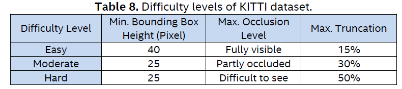
Accuracy Evaluation
We use the KITTI 3D object detection dataset [12] to evaluate the accuracy of the NN models. As Table 8 shows, there are three difficulty levels of this dataset.
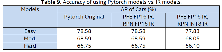
After integrating the IE into the PointPillars pipeline of SmallMunich [9], we can evaluate the accuracy for the three difficulty levels. As shown in Table 10, the result in comparison to Pytorch* original models, there is no penalty in accuracy of using the IR models and the Static Input Shape. It is also shown that the quantization of RPN model to INT8 only results in less than 1% accuracy loss.
Table 9 shows cars AP results on KITTI test 3D detection benchmark.
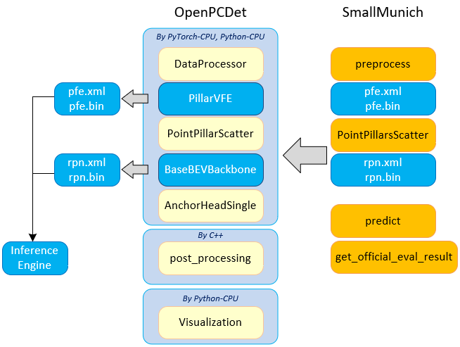
Migration from SmallMunich to OpenPCDet
The OpenPCDet is used as the demo application. Since we use the SmallMunich to generate the ONNX models, so we need to migrate not only the NN models (PFE and RPN) but also the non-DL processing from the SmallMunich code base to the OpenPCDet code base.
About 90% of the source codes of the SmallMunich and OpenPCDet are the same. Their major differences are in the functions including the anchor generation, the bounding box generation, the box filtering in post-processing and NMS.
After the migration of the source codes from SmallMunich to OpenPCDet, the OpenPCDet pipeline can generate the same results as that of the SmallMunich.
Profiling of the Pipeline
We run the pipeline on KITTI 3D object detection dataset, http://www.cvlibs.net/datasets/kitti/eval_object.php?obj_benchmark=3d. The 3D points are captured by Velodyne HDL-64E, which is a 64 channel lidar. It spins at 10 frames per second, capturing approximately 100K points per frame. We reduce the point number to around 20K per frame, by create_reduced_point_cloud() function based on SmallMunich [9] codebase.
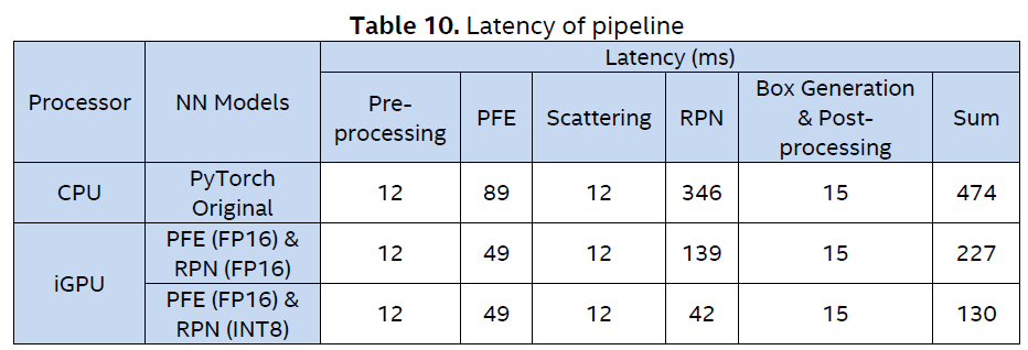
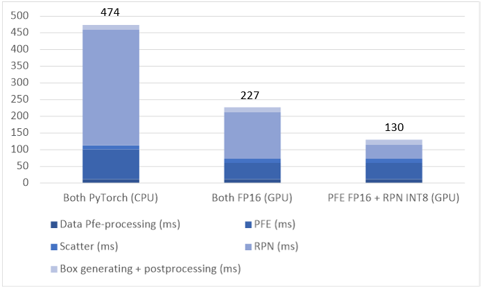
We evaluated the latency of the pipeline optimized by Section 5.3 on Intel® Core™ i7-1165G7 processor and the results are summarized in Table 10.
We further visualized the sum latencies by the bar chart in Figure 11. It shows that the NN model optimization and quantization by the OpenVINO™ toolkit can significantly accelerate the pipeline processing.
Three Pipeline Modes
As shown in Figure 12, the latencies for both PFE and RPN inferences have been significantly reduced compared to their original implementation. Next, we consider the further optimization of pipeline based on different performance targets.
We developed the below mentioned pipeline modes to meet different performance targets:
- Latency Mode: to achieve the shortest latency;
- Throughput Mode: to achieve the maximal throughput;
- Balanced Mode: to achieve the tradeoff between the latency and the throughput.
Latency Mode
In this mode, each step in the pipeline starts running right after the previous step is finished, i.e., these steps are executed seamlessly in the following sequence:
- At T0, starts pre-processing;
- At T1, calling infer() to let the IE to run the inference on PFE model;
- At T2, Scattering to map the 3D feature map to the 2D pseudo image;
- At T3, calling infer() to let the IE to run the inference on RPN model;
- At T4, starts post-processing.
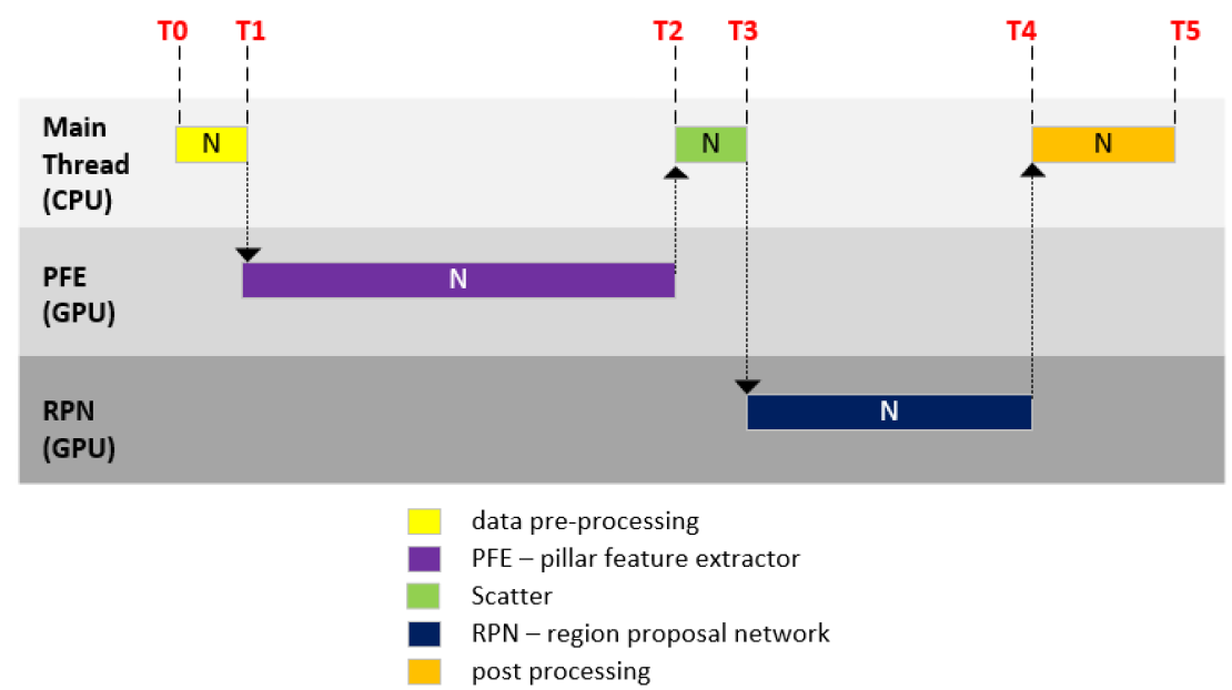
As Figure 13 shows, at one specific time, the pipeline only uses either CPU or iGPU. These two processors are exclusively used by the processing for one frame. These steps are executed seamlessly in sequence, thus the shortest latency is achieved.
Throughput Mode
The IE in the OpenVINO™ toolkit is capable of asynchronous processing with the API async_infer(). This means that the steps for one frame can be done with the steps for another frame in parallel.
In this mode, the main thread runs on the CPU which handles the pre-processing, scattering and post-processing. The inference using the PFE and RPN models run on the separated threads automatically created by the IE using async_infer() and these threads run in the iGPU.
Let’s take the N-th frame as an example to explain the processing in Figure 14.
- At T0, the main thread starts handling the pre-processing for the N-th frame;
- At T1, once notified by the IE that the (N-1)-th frame’s PFE inference is finished, the main thread starts 2 jobs:
- PFE inference for the N-th frame;
- Scattering for the (N-1)-th frame;
- At T2, when the scattering for the (N-1)-th frame is done, the main thread starts 3 jobs:
- RPN inference for the (N-1)-th frame;
- Post-processing for the (N-2)-th frame;
According to the profiling, the RPN inference for the (N-2)-th frame is already done at this time, meaning the post-processing for the same frame can start. - Pre-processing for the (N+1)-th frame;
Starts after the completion of the post-processing for the (N-2)-th frame.
- At T4, once notified by the IE that the N-th frame’s PFE inference is finished, the main thread starts 2 jobs:
- PFE inference for the (N+1)-th frame;
- Scattering for the N-th frame;
- At T5, when the scattering for the N-th frame is done, the main thread starts 3 jobs:
- RPN inference for the N-th frame;
- Post-processing for the (N-1)-th frame
According to the profiling, the RPN inference for the (N-1)-th frame is already done at this time, meaning the post-processing for the same frame can start. - Pre-processing for the (N+2)-th frame;
Starts after the completion of the post-processing for the (N-1)-th frame.
- At T7, once notified by the IE that the (N+1)-th frame’s PFE inference is finished, the main thread starts the scattering for the same frame, which is followed by the post-processing for the N-th frame at T8.

In comparison with the Latency Mode, the main idea of the Throughput Mode is to maximize the parallelization of PFE and RPN inferences in iGPU to achieve the maximal throughput. The loading of iGPU is quite high, about 95% in average.
However, this increases the latency for each frame (e.g., the N-th frame) due to:
- The inference latency for both PFE and RPN increases when they are run paralleled in iGPU;
- In the pipeline for the N-th frame, there are two waiting periods:
- The PFE inference has to wait for the completion of the PFE inference for the (N-1)-th frame, from T1 to T2;
- The post-processing has to wait for the completion of the scattering for the (N+1)-th frame, from T7 to T9.
The increased latency is the price that is paid for the parallelization of the PFE and RPN inferences.
Balanced Mode
This mode is used to achieve the tradeoff between the latency and the throughput.
Let’s take the N-th frame as an example to explain the processing in Figure 15.
- At T0, the main thread starts handling the pre-processing for the N-th frame;
- At T1, the main thread calls async_infer() to ask the IE to run PFE inference for the N-th frame;
- At T2, once notified the completion of RPN inference for the (N-1)-th frame, the main thread starts the post-processing for the (N-1)-th frame;
- At T3, once notified the completion of PFE inference for the N-th frame, the main thread starts the scattering for the N-th frame;
- At T4, after the scattering is done, the main thread starts 2 jobs:
- RPN inference for the N-th frame;
- Pre-processing for the (N+1)-th frame;
- At T6, once notified the completion of RPN inference for the N-th frame, the main thread starts post-processing on the N-th frame.

The loading of iGPU is 86% (compared with that of 95% in the Throughput Mode) due to the less parallelization of the PFE and RPN inferences.
Performance Evaluation Results
We evaluated the three modes of the PointPillars pipelines optimized by the OpenVINO™ toolkit on Intel® Core™ i7-1185GRE processor. The results are summarized in Table 11.
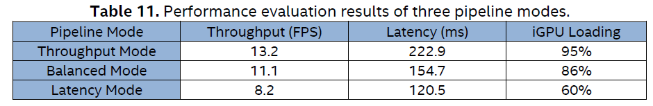
The different pipeline modes are designed based on the profiling results of each step (component) of the PointPillars pipeline.It is shown that the higher parallelization can obtain better throughput but worse latency.
The profiling results show the PFE inference takes the longest time, therefore we parallelize the rest of the steps of the pipeline with the PFE inference, for the Throughput Mode and the Balanced Mode.

Future Work
As future work, we want to continue exploring the trade-off between the processing speed and the accuracy. We will utilize the Intel distributed toolkits, for example:
- To quantize PFE model by POT in OpenVINO™ toolkit, and constrain the accuracy loss by the accuracy checker
- To refine and compress the PointPillars network by NNCF in OpenVINO™ toolkit, https://github.com/openvinotoolkit/nncf.
- To combine the PointPillars components as single one IR model by MO in OpenVINO™ toolkit.
Acronyms
For the purposes of the present document, the following acronyms apply:
Table 12. Acronyms
| AI | Artificial Intelligence |
| AP | Average Precision |
| CNN | Convolutional Neural Network |
| CUDA | Compute Unified Device Architecture |
| DL | Deep Learning |
| E2E | End-to-End |
| EU | Execution Unit |
| FP16 | Half-Precision Floating-Point Format (16 bits) |
| FP32 | Single-Precision Floating-Point Format (32 bits) |
| FPS | Frames Per Second |
| GPU | Graphics Processing Unit |
| IE | Inference Engine It is a set of C++ libraries providing a common API to deliver inference solutions on the platform of your choice: CPU, GPU, or VPU. For Intel® Distribution of OpenVINO™ toolkit, the IE binaries are delivered within release packages. |
| iGPU | Integrated Graphics Processing Unit |
| INT8 | Integer Format (8 bits) |
| IR | Intermedia Representation OpenVINO™ toolkit introduces its own format of graph representation and its own operation set. A graph is represented with two files: an XML file and a binary file. This representation is commonly referred to as the IR. |
| ML | Machine Learning |
| MO | Model Optimizer It is a cross-platform command-line tool that facilitates the transition between the training and deployment environment. It is delivered within Intel® Distribution of OpenVINO™ toolkit. |
| NMS | Non-Maximum Suppression |
| NN | Neural Network |
| ONN | Open Neural Network Exchange ONNX [1] is a representation format for DL models. ONNX allows AI developers easily transfer models between different frameworks that helps to choose the best combination for them. Today, PyTorch*, Caffe2*, Apache MXNet*, Microsoft Cognitive Toolkit* and other tools are developing ONNX support. |
| OpenVINO | Open Neural Network Exchange ONNX [1] is a representation format for DL models. ONNX allows AI developers easily transfer models between different frameworks that helps to choose the best combination for them. Today, PyTorch*, Caffe2*, Apache MXNet*, Microsoft Cognitive Toolkit* and other tools are developing ONNX support. |
| PFE | Pillar Feature Extractor |
| PFN | Pillar Feature Network |
| POT | Post-training Optimization Tool |
| RPN | Region Proposal Network |
| SKU | Stock Keeping Unit |
| TFLOPS | Tera (Trillion) Floating-point Operations Per Second |
| TOPS | Tera (Trillion) Operations Per Second |
Reference
[1] A. H. Lang, S. Vora, H. Caesar, L. Zhou, J. Yang and O. Beijbom, "PointPillars: Fast Encoders for Object Detection from Point Clouds," in IEEE/CVF Conference on Computer Vision and Pattern Recognition (CVPR), 2019.
[2] Intel, "OpenVINO overview," [Online]. Available: https://docs.openvinotoolkit.org/latest/index.html
[3] Intel, "TGLi7-1185GRE," [Online]. Available: https://ark.intel.com/content/www/us/en/ark/products/208082/intel-core-i7-1185gre-processor-12m-cache-up-to-4-40-ghz.html
[4] Intel, "TGLi7-1165G7," Intel, [Online]. Available: https://ark.intel.com/content/www/us/en/ark/products/208662/intel-core-i7-1165g7-processor-12m-cache-up-to-4-70-ghz.html
[5] "OpenPCDet project," [Online]. Available: https://github.com/open-mmlab/OpenPCDet
[6] "OpenMMLab project," [Online]. Available: https://github.com/open-mmlab
[7] Intel, "OpenVINO MO user guide," [Online]. Available: https://docs.openvinotoolkit.org/latest/openvino_docs_MO_DG_Deep_Learning_Model_Optimizer_DevGuide.html
[8] "ONNX," [Online]. Available: https://github.com/onnx/onnx
[9] "SmallMunich project," [Online]. Available: https://github.com/SmallMunich/nutonomy_pointpillars
[10] Intel, "OpenVINO POT user guide," [Online]. Available: https://docs.openvinotoolkit.org/latest/pot_README.html
[11] Intel, "IE integration guide," [Online]. Available: https://docs.openvinotoolkit.org/latest/openvino_docs_IE_DG_Integrate_with_customer_application_new_API.html
[12] KITTI, "KITTI 3D detection dataset," [Online]. Available: http://www.cvlibs.net/datasets/kitti/eval_object.php?obj_benchmark=3d
Annex A: Sample Codes of Quantization
The sample codes for the quantization by the POT API are the following:
class PointpillarsLoader(DataLoader):
    def __init__(self, config):
       if not isinstance(config, Dict):
         config = Dict(config)
       super().__init__(config)
       self._image_size = config.image_size
       self._img_ids = sorted(os.listdir(config.data_source))
    def __getitem__(self, index):
      """
      Returns annotation and image (and optionally image metadata) at
      the specified index.
      Possible formats:
      (img_id, img_annotation), image
      (img_id, img_annotation), image, image_metadata
      """
      if index >= len(self):
            raise IndexError
      image_path = os.path.join(self.config.data_source,
      self._img_ids[index])
      img = np.fromfile(image_path, dtype=np.float32).reshape(64,496,432)
      annotation_np = {'184': np.zeros((1, 248, 216, 14), dtype=np.float32),
                       '185': np.zeros((1,248,216,2), dtype=np.float32),
                       '187': np.zeros((1,248,216,4), dtype=np.float32)}
      annotation = (index, annotation_np)
      return annotation, img
  def __len__(self):
     """ Returns size of the dataset """
     return len(self._img_ids)
def main():
    model_config = Dict({
         'model_name': 'pointpillars',
         'model': '<your_folder>/rpn.xml',
         'weights': '<your_folder>/rpn.bin'
})

  engine_config = Dict({
     'device': 'CPU',
     'stat_requests_number': 4,
     'eval_requests_number': 4
  })
  dataset_config = Dict({
      'data_source': '<your_data_source>',
      'image_size': 200
  })
  algorithms = [
      {
          'name': 'DefaultQuantization',
          'params': {
                  'target_device': 'CPU',
                  'preset': 'performance',
                  'stat_subset_size': 100
      }
    }
  ]
  # Step 1: Load the model.
  model = load_model(model_config)

  # Step 2: Initialize the data loader.
  data_loader = PointpillarsLoader(dataset_config)

  # Step 3 (Optional. Required for AccuracyAwareQuantization): Initialize the metric.
  #metric = MeanIOU(num_classes=21)

  # Step 4: Initialize the engine for metric calculation and statistics collection.
  engine = IEEngine(config=engine_config,
                    data_loader=data_loader)

  # Step 5: Create a pipeline of compression algorithms.
  pipeline = create_pipeline(algorithms, engine)

  # Step 6: Execute the pipeline.
  compressed_model = pipeline.run(model)

  # Step 7 (Optional): Compress model weights to quantized precision
  # in order to reduce the size of final .bin file.
  compress_model_weights(compressed_model)

  # Step 8: Save the compressed model to the desired path.
  save_model(compressed_model, os.path.join(os.path.curdir, 'optimized'))

if __name__ == '__main__':
main()