Systematically Search Model Architectures with SigOpt
Ellick Chan, head of Intel® AI Academy, University Relations and Research,
and Barrett Williams, SigOpt® product marketing lead
@IntelDevTools
Get the Latest on All Things CODE
Sign Up
Neural architecture search (NAS) is a modern technique to find optimized neural networks (NN) for a given task, such as image classification, through structural iteration and permutation. Network parameters like the depth of the network, number of convolutional filters, pooling, epochs, and learning rate can substantially impact a network’s accuracy, inference throughput, and latency for a given dataset.
The search space for these parameters is large, so NAS can take many compute hours to train. This article shows how you can use smarter search algorithms provided by SigOpt paired with raw cluster computing power provided by Ray Tune to accelerate this process. A simple example is used so that you can apply this technique to your own workflows.
To illustrate the core concept of NAS, consider the original network shown in column a in Figure 1. This reference network consists of a single input layer followed by one or more copies of Block 1. Block 1 is based on a convolution pooling motif consisting of 3×3 convolutions with 32 filters, optionally followed by a pooling operation. This pattern continues with one or more copies of Block 2, similarly composed of 32 3×3 convolutional filters. These convolutional blocks are then flattened to a vector, processed through a fully connected layer, and topped off with a softmax function for final classification.
NAS helps the data scientist test a variety of permutations of a reference architecture. Column b in Figure 1 shows one option called depth scaling, in which Block 2 is repeated to increase the effective depth of the network. For good measure, we also optionally add another fully connected layer of 1024 neurons. In this tutorial, the two fully connected layers are the same size, but they can be different sizes in your application.
Column c in Figure 1 shows width scaling, in which the depth of the network remains constant but parameters on the operators are varied. In this case, we reduce the number of convolutions in L1 (layer 1) from 32 to 16, and increase the number of convolutions in L2 from 32 to 64. We also make the fully connected layer wider, going from 1024 to 2048. Note that NAS does not have to search for all parameters at once. It is possible to optimize one parameter at a time and fix the others, or if your optimizer is intelligent like SigOpt, it is both possible and more efficient to strategically update multiple parameters at once to find the best network architecture more quickly.
Column d in Figure 1 explores one more dimension by challenging our assumption of using 3×3 filters. Instead, we substitute the filters in Block 1 with 5×5 filters and Block 2 with 7×7 filters. This can help the performance of certain models and datasets, depending on data characteristics and input image resolution.
By now, it’s fairly clear that even with a simple example, there are a combinatorially large number of NN parameters to customize and explore. In the rest of this article, we show you how to use SigOpt and Ray Tune to fine tune the space of simple NN used to classify images in the classic CIFAR10 dataset.
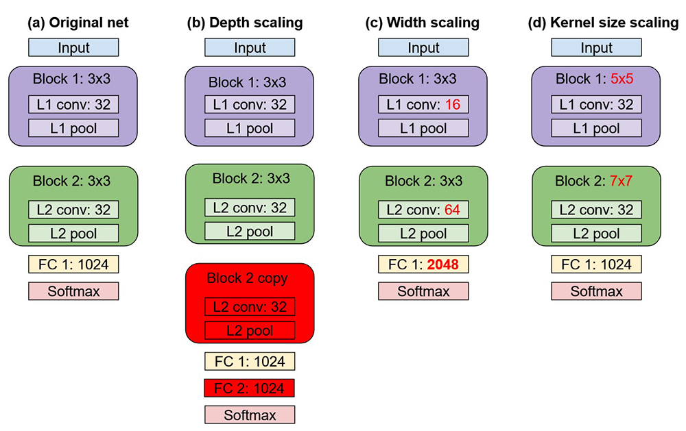
Figure 1. Network variations used in this tutorial
Overall Workflow
- Define an NN training task. Choose a dataset and a model template (for example, the CIFAR-10 convolutional neural net [CNN]), and then define the parameters to tune (for example, number of layers or filters).
- Apply Ray Tune to search for a preliminary set of model parameters.
- Adapt the search algorithm to SigOpt to get better parameters more efficiently.
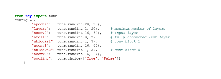
Parameterizing the Model
For the purposes of this article, define an NN training task as a convolutional network with one or more convolutional blocks. We use the CIFAR-10 dataset and the Keras* API from TensorFlow*.
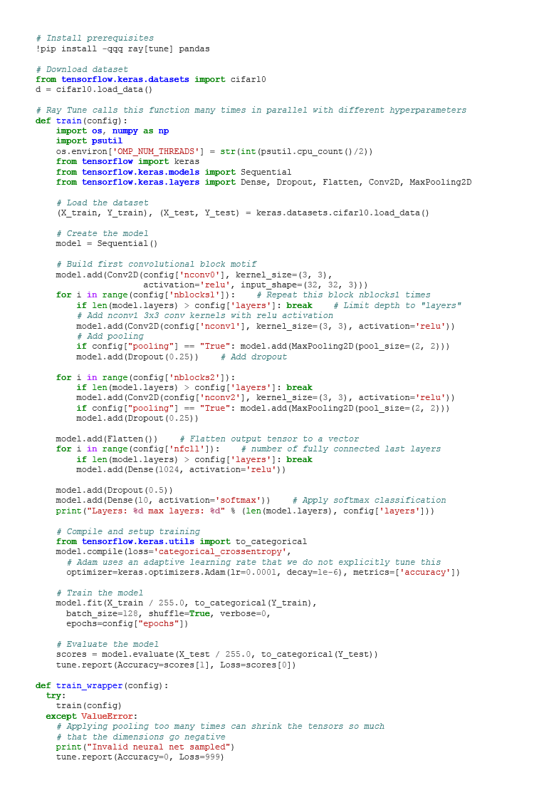
To parameterize the model, we define the following:
- Epochs: Number of epochs to train a model
- Layers: Maximum number of layers of the desired model (subsequent layers are pruned)
- Nconv0: Number of 3×3 convolution filters for the input layer
- Nfcll: Number of fully connected last layers with 1,024 neurons each
- Pooling: Global setting to enable or disable pooling in convolution blocks 1 and 2
- Nblocks1: Number of copies of convolution block 1
- Nconv1: Number of 3×3 convolution filters for convolution blocks 1 and 2
- Nblocks2: Number of copies of convolution block 2
- Nconv2: Number of 3×3 convolution filters for block 2
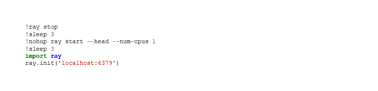
To be consistent for deploying clusters in Part 2 (to be published later), start Ray Tune from the command line. If you are running on a single node, the following commands are not necessary:
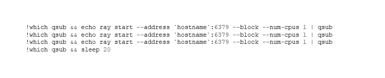
If you are running on a cluster such as Intel® DevCloud that uses a job scheduler (such as the Portable Batch System), the following commands start worker processes on multiple nodes:
Finally, set the parameters:
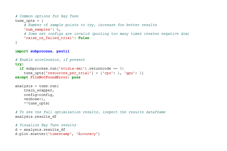
Apply Ray Tune
Ray Tune is a Python* library that facilitates scaled experimentation, as well as hyperparameter optimization via SigOpt, which allows multiple worker nodes to explore the search space in parallel. A naïve grid search of our defined parameter space would explore nearly 1.2 billion possible configurations.1 This article shows how to use random search to speed up this process, and then follows up with a smarter guided search using SigOpt, effectively comparing the performance and output of the two approaches.
For Ray Tune, the most important inputs are the function to optimize (train) and the search space for the parameters (config). We defined both of these earlier and provide the corresponding code below. Other options include a choice of search algorithm and scheduler for more guided searches.
1 This estimate is derived from 10*20*(64-16)*3*3*(64-16)*3*(64-16)*2.
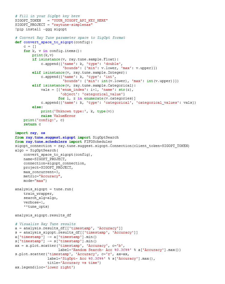
Integrate with SigOpt
You can create an account, which gives you access to an API key that you can use in your Google CoLaboratory* notebook or Jupyter* Notebook for the Intel DevCloud.
Interpret SigOpt Results
The previous example used a limited number of sample points to allow the experiment to complete quickly. If more data points are sampled, you might see a figure like the one shown in Figure 2, which illustrates that the SigOpt directed search finds better solutions more efficiently than random search.
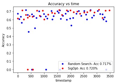
Figure 2. SigOpt directed search vs. random search
SigOpt helps data scientists understand which parameters matter most for their NAS. The number of epochs has the biggest influence on the accuracy of the network, followed by pooling layers, and then the number of convolutional filters (Figure 3). SigOpt searches this space intelligently to find the best values more efficiently.
To help data scientists understand the influence of various parameters, SigOpt visualizes the relative parameter importance with respect to the points sampled. Note that this is a bit of a biased sample as the points are chosen intelligently by the optimizer (instead of at random).
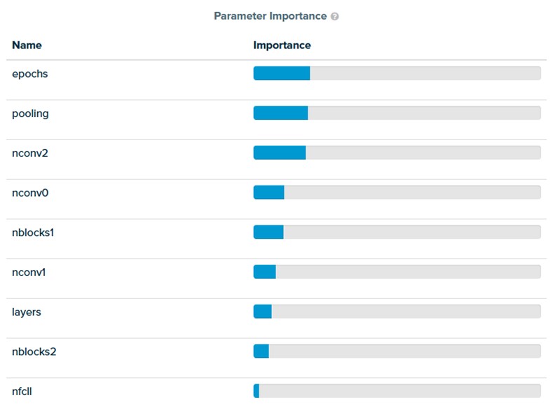
Figure 3. Determine which parameters matter the most
Given the relative importance of the parameters, we examine the relationship between convolutional filter parameters nconv0 and nconv1 and find that this particular problem prefers around 50 filters for nconv0 and a small number of filters for nconv1 (Figure 4). Any pair of variables can be visualized in this plot.
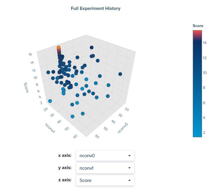
Figure 4. Visualizing the relationship between parameters
A parallel coordinates plot shows the trajectory of the parameter search (Figure 5). In this case, the highest scores are obtained with a larger number of epochs, pooling, and different combinations of layer parameters. This plot shows what this particular problem prefers. If the dataset or objective is changed, the preferred parameters may differ.
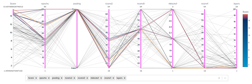
Figure 5. Trajectory of the parameter search
Understanding the relationships between the parameters helps data scientists better optimize parameter values for the problem and better manage tradeoffs. Start optimizing, tracking, and systematizing today.