Introduction
Reservoir simulators typically use Krylov methods for solving the systems of linear equations that appear at every Newton iteration. One key step in most Krylov methods, executed at every linear iteration, involves orthogonalizing a given vector against a set of (already) orthogonal vectors. The linear solver used in the reservoir simulator we worked on implements the Orthomin method and utilizes the Modified Gram-Schmidt algorithm to execute this operation. This process has, for some simulations, a high contribution to the total computation time of the linear solver. Therefore, performance optimizations on this portion of the code may provide performance improvements for the overall simulation.
Figure 1 shows the percentage of total time spent on the Linear Solver and in the Gram-Schmidt kernel for several parallel simulations. The percentage of time spent on the Modified Gram-Schmidt method inside the linear is a hotspot on the simulator, ranging from 6% on Case 1 up to 51% on the Case 2. This result demonstrates the importance of trying to optimize this computation kernel.

Figure 1. Gram-Schmidt and Linear solver total time percentage for parallel simulations. The number of MPI processes used in the run is indicated between parentheses.
This work describes an implementation of the Classic Gram-Schmidt method on the linear solver of a reservoir simulator under development. The implementation is based on the work developed by João Zanardi, a Graduate Student from Rio de Janeiro State University (UERJ) during his internship at Intel Labs (Santa Clara, USA). The proposed implementation of the Classic Gram-Schmidt method provides performance benefits by improving data locality in cache during the linear algebra operations and by reducing the number of collective MPI calls.
We achieved up to 1.7x performance speedup in total simulation time with our optimized Classic Gram-Schmidt when compared to the current implementation of the Modified Gram-Schmidt. However, the Classic Gram-Schmidt implementation does not over perform the current implementation in all cases. It seems that the part of the vectors associated to each thread needs to have a minimum size in order for the Classic Gram-Schmidt to be advantageous.
In Section 1 we describe the two versions of the Gram-Schmidt method, leaving for Section 2 a more detailed explanation of certain aspects of how the Classic version was implemented in our reservoir simulator. Section 3 presents the results of the tests we made, starting with a microbenchmark program specifically written to test the Gram-Schmidt kernel in isolation, then comparing the performance of the two approaches for the Linear Solver alone on matrices dumped from the reservoir simulator and finally testing the methods on actual simulation runs. Section 4 provides the conclusions of this study.
1. Description of the Classic and Modified Gram-Schmidt Methods
Listing 1 shows the current implementation of the Modified Gram-Schmidt method used in the reservoir simulator linear solver. Vector qj is orthogonalized with respect to vectors qi, i = 0 to j − 1, while vector dj is updated as a linear combination of vectors di, i = 0 to j – 1. For applications of interest in this work, qj and dj are vectors whose size can reach several million, while j, the number of vectors in the base, is a small number, typically a few dozen. For each pair of vectors qi and qj it is necessary to compute an inner product (line 9) through the brackets operator of the object ip. Then the scalar alpha is stored and vectors qj and dj are updated in lines 10 and 11.
V* q = &qv[0];
V* d = &dv[0];
V& qj = q[j];
V& dj = d[j];
for( int i = 0; i < j; i++ )
{
        const V& qi = q[i];
        const V& di = d[i];
        const double alpha = ip( qj, qi );
        qj -= alpha * qi;
        dj -= alpha * di;
}
Listing 1. Source code for the Modified Gram-Schmidt utilized on the current linear solver.
We can see in Listing 1 that the inner product and update (axpy) on lines 9, 10 and 11 are BLAS level one operations (vector operations) and, therefore, they have low arithmetic intensity, with their performance limited by the memory bandwidth. The Modified Gram-Schmidt method has a loop dependence since every pass on the loop updates the qj vector (line 10) to be used in the inner product of the next pass (line 9), which leaves no room for data reuse in order to improve data locality.
In order to overcome this limitation, one possibility is to use the Classic Gram-Schmidt method, as discussed in several references in the literature (e.g. 1 and 2). The Classic GS method is also the default option in the well-known PETSc library, as well as other solver libraries, and it is implemented in other reservoir simulators. Listing 2 presents the algorithm. The inner products needed to calculate the alpha values are performed before the qj vector is updated, removing the recurrence observed in the Modified version. All three loops in the algorithm can be recast as matrix-vector multiplications and, therefore, BLAS2 operations can be used, with better memory access. More specifically, let Q be the matrix whose columns are the vectors qi, i = 0 to j − 1, then the loop in lines 5 to 9 calculates
alpha_vec = QT qj, (1.1)
where alpha_vec is a size j – 1 vector containing the alpha values, while the loop in lines 11 to 15 calculates
qj = qj − Q alpha_vec. (1.2)
Similarly, if D denotes the matrix whose columns are the di vectors, the loop in lines 17 to 21 calculates
dj = dj − D alpha_vec. (1.3)
In order to realize the potential performance benefits of interpreting the orthogonalization and updating as BLAS2 operations, as given by, and, blocking has to be used. The objective of blocking techniques is to organize data memory accesses. The idea is to load a small subset of a large dataset into the cache and then to work on this block of data without the need to bring it back to cache. By using/reusing the data already in cache, we reduce the need to go to memory, thus reducing memory bandwidth pressure 6.
Our implementation of the blocking technique will be shown in the next section, where our implementation in the simulator is detailed. It will also be clear that switching to BLAS2 results in less communication when running in parallel.
V* q = &qv[0];
V* d = &dv[0];
V& qj = q[j];
V& dj = d[j];
for( int i = 0; i < j; i++ )
{
   const V& qi = q[i];
   alpha[i] = ip( qj, qi );
}

for( int i = 0; i < j; i++ )
{
   const V& qi = q[i];
   qj -= alpha[i] * qi;
}

for( int i = 0; i < j; i++ )
{
   const V& di = d[i];
   dj -= alpha[i] * di;
}
Listing 2. Source code for the Classic Gram-Schmidt method without blocking.
Note that the Modified version could be rewritten in such way that the update of dj is recast as matrix-vector calculation. In fact, line 11 of Listing 1 is independent of the other calculations in the same loop and could be isolated in a separated loop equal to the loop in lines 17 to 21 of Listing 2. We had tested this alternative implementation of the Modified version, but our preliminary results indicated that the speedup obtained is always very close to or lower to what it can be obtained with the Classic version and we decided to not pursue on any further investigation along those lines.
It is very important to note that the Classic and Modified versions are not equivalent and it is a well-known fact that, in the presence of round-off errors, Classic GS is less stable than Modified GS 5, with the consequence that it is more prone to loss of orthogonalization in the resulting vector basis. To what extent this is an issue for its application to Krylov methods has been discussed in the literature 1, 2, 3, 4, but apparently, it does not seem to be particularly serious, considering that, as alluded above, it is successfully applied in several solvers. This seems to be corroborated by our experience with the implementation in the simulator, as it will be shown in Section 3.
2. Implementation of Classic Gram-Schmidt on the Simulator
In order to explore the potential of data reuse introduced by recasting the calculations as BLAS2 operations, it is necessary to block the matrix-vector multiplications. Figure 2 depicts the blocking strategy for the matrix-vector multiplication. The contribution of each chunk of qj is calculated for all qi’s, allowing reuse of qj, improving memory access. Listing 3 shows the corresponding code for calculating the alpha vector using this blocking strategy. The Intel Compiler provides a set of pragmas to ensure vectorization 7. The reservoir simulator already made use of pragmas on several computational kernels and we also add pragmas to ensure vectorization.

Figure 2. Representation of the blocking strategy used to improve data traffic for.
const int chunkSize = 2048;
for(int k = 0; k < size; k += chunkSize)
{
    for( int i = 0; i < j; i++ )
    {
        double v = 0.0;
#pragma simd reduction(+:v)
       for(int kk = 0; kk < chunkSize; kk++)
       {
            v += qj[k + kk] * Q[i][k + kk];
       }
       alpha[i] += v;
    }
}
Listing 3. Source code for local computation of the alpha factor using a matrix-vector blocked operation.
Careful examination of Figure 2 and Listing 3 reveals that implementation of the Classic method has another opportunity to improve performance, in addition to blocking. The alpha factors are calculated without using the inner product operator, reducing MPI communication calls, as only a single MPI All reduce call on the entire alpha vector is required. Note that in the Modified version, an inner product has to be done for each alpha due to the loop recurrence and, consequently, a reduction is triggered for each i in the loop in line 5 of Listing 1.
Similarly, blocking is also required to reduce data traffic for calculations and. Figure 3 and Listing 4 are the counterparts of Figure 2 and Listing 3 for the updating operations, showing how the blocking strategy is implemented in that case. The updating of each chunk of qj is calculated for all qi’s, allowing reuse of qj, improving memory access.

Figure 3. Representation of the blocking strategy used to improve data traffic for. The same strategy can also be applied to.
const int chunkSize = 2048;
for(int k = 0; k < size; k += chunkSize)
{
    double temp[chunkSize];
    for( int i = begin; i < j; i++ )
    {
#pragma simd vectorlength(chunkSize)
        for(int kk = 0; kk < chunkSize; kk++)
        {
            temp[kk] += alpha[i] * Q[i][k + kk];
        }
    }
#pragma simd vectorlength(chunkSize)
    for(int kk = 0; kk < chunkSize; kk++)
    {
        qj[k + kk] -= temp[kk];
    }
}
Listing 4. Source code for the update of the vectors qj and dj using a modified matrix-vector blocked operation.
The optimizations used on this work are focused on our hardware used on production (Sandy Bridge). This kernel may show better performance on newer Intel® processors (Broadwell) that supports FMA (Fused Multiply Add) instructions and improved support for vectorization.
3. Tests
3.1 System Configuration
We performed all experiments on a workstation with two Intel® Xeon® processors and 128GB of DDR3 1600MHz memory. Table 1 shows the configurations of the processors used. All experiments were executed using Linux* RedHat 6 with kernel 2.6.32. Intel® MPI Library 5.0.1 and Intel® C++ Compiler XE 14.0.4 with compilation flags -O3, -fp-model fast and -vec were used.
Table 1. Description of the hardware used in the experiments.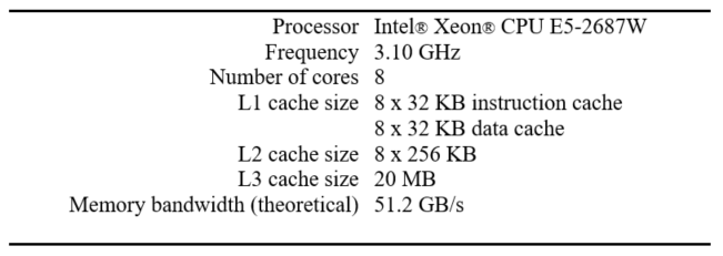
3.2 Performance Comparison with a Microbenchmark
To evaluate the performance relation between the size of the vectors and the number of processes, we developed a microbenchmark that initializes a set of vectors in parallel and executes only the orthogonalization process, so that we can look directly to the Gram-Schmidt performance without any influences from the linear solver.
Table 2. Performance improvement of the Classic Gram-Schmidt over the Modified version in the microbenchmark for several vector sizes and the number of processes. Greater than one means Classic is faster than Modified, the higher the better.
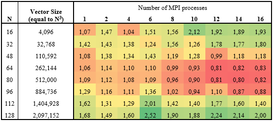
Table 2 shows the performance improvement of the Classic method over the Modified version of the Gram-Schmidt method. In the table rows, we vary the qj and dj vector sizes and in the table columns, we vary the number of MPI processes used for parallel processing. Vector sizes were generated based on the number of cells of a regular N x N x N grid. The total number of vectors was 32 and chunk size was 2048. The value for the chunk size was obtained by performing a series of experiments with the microbenchmark program. Figure 4 shows the results of one such experiment performed in an early phase of this study, showing the performance benefits of increasing chunk size up to 1024. Further experiments determine that 2048 was slightly better. In all results to be presented in the next sections, this was the chunk size value used. It is expected that the ideal chunk size will depend on the machine features, such as cache size.
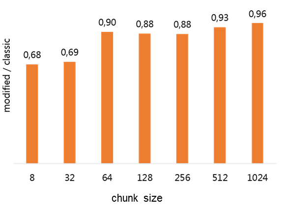
Figure 4. Ratio between the times for the Modified and Classic Gram-Schmidt implementations as a function of chunk size. Greater than one means Classic is faster than Modified, the higher the better. Vector size is 256 x 1024 and 32 is the number of vectors.
From Table 2 one can notice that Classic can be more than twice as fast as the Modified for the largest vectors. On the other hand, for vectors of intermediate size, Modified is faster when eight or more processors are used. For all numbers of processes, Classic loses performance, relatively to Modified, for the intermediate size vectors. So far, we have not reached a conclusion about the reason for this performance loss. Apparently, there is a minimum size for the part of the vector associated with a process in order to have the advantage when using Classic Gram-Schmidt.
3.3 Microbenchmark Profiling with Intel® VTune™ Amplifier and Intel® Trace Analyzer
To evaluate the reduction in communication time between the current implementation of the Modified method and our Blocked Classic method we utilized the microbenchmark and the Intel Trace Analyzer tool in the Linux operating system. To do so, we recompiled our microbenchmark by linking with appropriate Intel Trace Analyzer libraries.
We run the microbenchmark by varying the size of the vectors from 4,096 to 2,097,152 in the same execution with 16 MPI processes. Figure 5 shows the percentage of time spent with MPI communication in relation to the total time for the current implementation of the Modified method. In Figure 6 we have the percentage of time spent with MPI communication in relation to the total time for our implementation of the Classic method. Comparing the two figures we can notice a reduction of the percentage of time spends with MPI from 15.3% to 1.7%, which implies a reduction of time in the order of 15x in the Classic method.
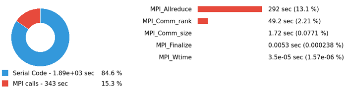
Figure 5. Ratio of all MPI calls to the rest of the code in the application for the Modified method.
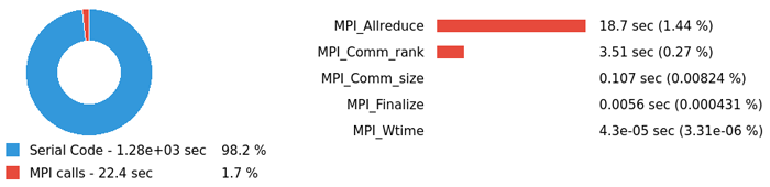
Figure 6. Ratio of all MPI calls to the rest of the code in the application for the Classic method.
In addition, we also use an Intel VTune Amplifier tool to check the vectorization of the Modified method and our implementation of the Classic method. For this, we executed the microbenchmark with a single process and with vectors of sizes 2,097,152 using the General Exploration Analysis type on Intel VTune Amplifier.
In Figure 7 and Figure 8, we have images from the Intel VTune Amplifier focusing on the code generated to vector update operations (AXPY) for Modified and Classic methods, respectively. These figures show that in both versions of the method the compiler was able to generate versions of the code with vectorization.

Figure 7. Update vector section generated code from the Intel VTune Amplifier running the Modified method.
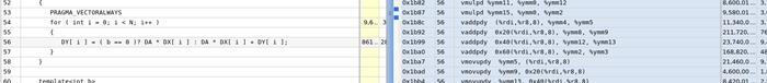
Figure 8. Update vector section generated code from the Intel VTune Amplifier running Classic method.
In Figure 9 and Figure 10, we have the initial section of the Bottom-Up view in General Exploration Analysis for the Modified and Classic methods, respectively. In Figure 9, the code section responsible for updating the vectors (AXPY) is marked with a high incidence of LLC Hits. According to the VTune documentation: "The LLC (last level cache) is the last and highest latency, level in the memory hierarchy before the main memory (DRAM). While LLC hits are met much faster than DRAM hits, they can still incur a significant performance penalty. This metric also includes consistency penalties for shared data”. Figure 10 shows that our Classic method implementation does not present a high incidence of LLC, showing that the blocking method implemented was efficient to maintain the data at the L1 and L2 cache levels.
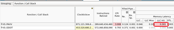
Figure 9. Initial section of the General Exploration Analysis Bottom-Up view from VTune Amplifier executing the Modified method.
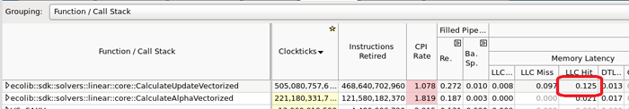
Figure 10. Initial section of the General Exploration Analysis Bottom-Up view from VTune Amplifier executing the Classic method.
3.4 Experiments with Extracted Matrices
In order to understand how the two methods compare within the overall linear solver, we used two matrices extracted from simulations and compare the linear solve performance using the Classic and Modified versions with 1, 2, 4, 8 and 16 processes. In the first case (Case 3) vector size is 2,479,544 and in the second (Case 2) 4,385,381. The number of iterations obtained by both methods was the same in all cases.

Figure 11. Time ratio of the Classic method over the Modified for matrices extracted from Case 3. Greater than one means Classic was faster, the higher the better.
Figure 11 and Figure 12 show the performance improvements for the two cases for the different numbers of processes. In all configurations, the Classic version yields substantial gains in the Gram-Schmidt kernel, ranging from 1.5x to 2.5x when compared to the Modified one. The corresponding benefit in the overall linear solution is also very expressive, ranging from 1.2x to 1.5x for Case 2 and from 1.1x to 1.3x for Case 3.

Figure 12. Time ratio of the Classic method over the Modified for matrices extracted from Case 2. Greater than one means Classic was faster, the higher the better.
For the Case 3 matrix with 16 MPI processes, we use the Intel® VTune™ Amplifier XE 2015 tool in Hotspot Analysis mode to evaluate the communication reduction. In Figure 13 and Figure 14 we show the profile of the Modified and the Classic methods, respectively. The MPI_Allreduce calls within the inner product method for the Modified version take 36 seconds of CPU time (6% of orthogonalization time). The Classic method profile shows 6.28 seconds spent on MPI_Allreduce calls (2% of orthogonalization of time), showing a large reduction in communication time. However, in this scenario of a small number of processes the communication does not represent a major portion of the orthogonalization time and, therefore, it does not have a big impact on the overall performance. This is likely to change when increasing the number of processes and running in cluster environments where communication takes place via the communication network.
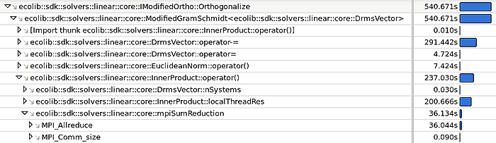
Figure 13. Modified Gram-Schmidt benchmark profile from the Intel® VTune™ Amplifier XE 2015 for the Ostra matrix with 16 MPI processes.
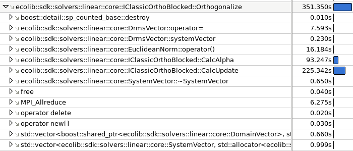
Figure 14. Classic Gram-Schmidt benchmark profile from the Intel VTune Amplifier XE 2015 for the Ostra matrix with 16 MPI processes.
3.5 Performance Comparison with Full Simulations
In order to assess the impact of replacing the Modified Gram-Schmidt method by the Classic one in the performance of actual simulation runs, seven test cases were executed. Table 2 contains the main features of the cases. Note that vector sizes for most of the cases are in the intermediate range where Table 2 shows the least performance for the Classic when compared with the Modified, the exceptions being Case 2, which is beyond the largest sizes in Table 2, and Case 1, which is in the range of the smallest sizes.
Table 3. Main features for the seven test cases.

The number of time steps, cuts and linear and nonlinear iterations taken for each case with the two Gram-Schmidt implementations is shown in Table 2. In five out of the seven cases, the performance of the Modified and Classic is very close. For Case 2 and Case 4, Classic performs clearly better, particularly in Case 2 where the number of linear iterations decreases 16%.
Table 4. Numerical data for the seven test cases. Inc is the relative increment from Modified to Classic (negative when Classic took less time steps, cuts, and iterations).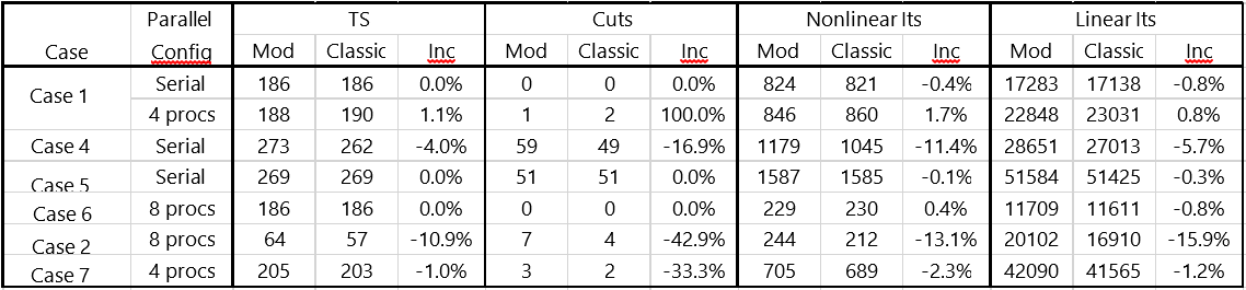
Figure 9 shows the performance gains provided by using the Gram-Schmidt Classic method for the three serial runs. The performance of both methods is very close for Case 5 and Case 4, while there is around 10% improvement in the Gram-Schmidt kernel for Case 1. Those results seem to be in line with the findings from the microbenchmark program, as Case 1 vector size is in the small range where Table 2 shows benefits for the Classic version. The improvement in Gram-Schmidt does not extend to the Linear Solver whose performance is almost the same with both methods.
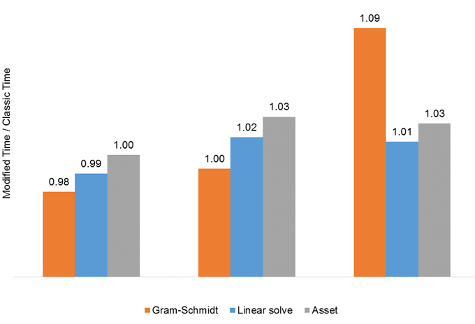
Figure 15. Time ratio of Classic Gram-Schmidt over Modified for the serial runs.
Figure 10 is similar to Figure 9 for the parallel runs. Case 7 shows a slight improvement with the Classic, while Case 4 and Case 1 show degradation in performance, particularly the latter, where time for the Modified is almost 20% smaller. The impact of those differences in Linear Solver and Asset time is minor. For Case 2, there is a substantial improvement in performance of the orthogonalization, with Classic being 2.8x faster. For this case, the benefits in Gram-Schmidt translate into a noteworthy improvement in both Linear Solver and Asset time, making the full simulation almost 1.7x faster. This is due both to the fact that vectors are very large and, therefore, Classic is supposed to over perform Modified by a large amount (see Table 2), as well as to improvement in linear and nonlinear iterations resulting from changing the orthogonalization algorithm. It is also important to note that Gram-Schmidt contributes with around half of the total simulation time for Case 2 (see Figure 16), which makes any benefits in this kernel to result in much clear improvements in total simulation time.
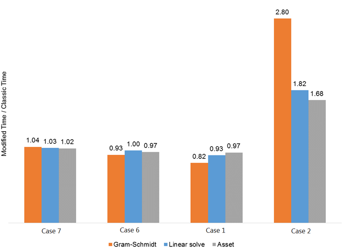
Figure 16. Time ratio of Classic Gram-Schmidt over Modified for the parallel runs.
4. Conclusions
The Classic Gram-Schmidt method was implemented in the reservoir simulator linear solver, using a blocking strategy for achieving better memory access. From the tests we made, the following conclusions can be taken:
- The new implementation provides a substantial performance improvement over the current one, based on the Modified Gram-Schmidt algorithm, for large problems where the orthogonalization step takes a considerable share of total simulation time. Typically, this will be the case when the number of linear iterations to solve each system is big, making the Krylov basis large. Outside of this class of problems, the performance is either close to or slightly worse than the current implementation.
- Using a performance analysis tool, we could observe a substantial reduction in communication time when using the Classic version. For the hardware configuration we used, it does not translate into a large benefit for the overall procedure, as the tests were executed in a workstation and parallelization was limited to at most 16 processes. It is expected that, for parallel runs in cluster environments with a large number of processes, the reduction in communication costs will become important to ensure good performance and parallel scalability.
- Despite known to be less stable than the Modified version, we have not noticed any degradation in convergence of the Krylov method when switching to the Classic version in our test cases. In fact, convergence for the Classic was even better than Modified in two out of the seven actual simulation models we ran.
- The blocking strategy adopted in the implementation depends on a parameter, the chunk size, which is hardware dependent. The study does not allow to say to what extent tuning this parameter to a specific hardware is crucial to obtain adequate levels of performance, as one single machine configuration was used in all tests.
- Experiments with a microbenchmark program focused on the Gram-Schmidt kernel showed a decrease in the performance of the Classic relative to the Modified for intermediate vector sizes. The results obtained for full simulations seem to corroborate those findings. At the moment, we have not found any consistent explanation for this phenomenon, although it seems to be related to the division of work per thread or process. It is also still unclear if it is possible to avoid the performance downgrade of Classic Gram-Schmidt (relative to the Modified) by tuning implementation.
References
- Frank, J. & Vuik, C., Parallel Implementation of a Multiblock Method with Approximate Subdomain Solution, Applied Numerical Mathematics, 30, pages 403-423, 1999.
- Frayssé, V., Giraud, L., Gratton, S. & Langou, J., Algorithm 842: A Set of GMRES Routines for Real and Complex Arithmetics on High Performance Computers, ACM Transactions on Mathematical Software, 31, pages 228-238, 2005.
- Giraud, L., Langou, J. & Rozloznik, M., The Loss of Orthogonality in the Gram-Schmidt Orthogonalization Process, Computers and Mathematics with Applications, 50, pages 1069-1075, 2005.
- Greenbaum, A., Rozloznik, M. & Strakos, Z., Numerical Behaviour of the Modified Gram-Schmidt GMRES Implementation, BIT, 37, pages 706-719, 1997.
- Golub, G.H. & Van Loan, C.F., Matrix Computations, Third Edition, The Johns Hopkins University Press, Baltimore and London, 1996.
- Cache Blocking Techniques, https://software.intel.com/content/www/us/en/develop/articles/cache-blocking-techniques.html accessed on 16/12/2016.
- Improve Performance with Vectorization, https://software.intel.com/content/www/us/en/develop/articles/improve-performance-with-vectorization.html.