Identify Plant Anatomy Using the Intel® Distribution of OpenVINO™ Toolkit

Introduction

This project uses an algorithm for the easy identification or classification of plant species via a mobile or web application. The entire system is an intelligent framework that enables users to identify a plant via a smartphone application – users merely need to open the app, click a picture, and view the result. Input for the system can be either an image or live video feed of the plant species, and the result is in the form of a bounding box with the name of the plant and the accuracy of the identification. Just clicking the photo produces the name or possible suggestions.

Figure 1. Plant anatomy detection using the Intel® Distribution of OpenVINO™ toolkit

Use Case for the Application

Millions of plant species exist in the world, many of them unknown. For the proper conservation and extraction of valuable insights, one must first know their scientific names. Once the name is known, features of each plant species are extracted by classifying them into family, class, genera, etc. The application can be a helpful for modern-day taxonomists, as well as naturalists and enthusiasts.

This article examines how the solution is built using deep learning and computer vision algorithms powered by the Intel® Distribution of OpenVINO™ toolkit Model Optimizer.

Overview and Architecture

As illustrated above, the primary objective of the project is to classify plant species correctly and with the utmost precision. The output of the model is the correctly classified name of the species. The input can be an image, video, or live camera feed of a flower, fruit, or leaf of the plant to identify.

The overall architecture flow is as follows:

1. Web Crawler (Gather Data)
   Write a Python* script to generate image from the Google Images* search service
2. LabelImg (Generate train and test data)
   Create labelled .xml files for the image data and then generate the .cvs files for training and testing along with the TensorFlow* record files
3. Intel® Optimization for TensorFlow
   Train the classifier using the Intel Optimization for TensorFlow and create a model. Optimize the model to create the .xml and .bin files
4. Intel Distribution of OpenVINO toolkit
   The Intel Distribution of OpenVINO toolkit Model Optimizer generates the .xml and .bin files to be used for inference

Further explanation of the steps as mentioned above are as follows:

1. Generate the data for training and testing the classifications from Google Images* search service. The optimal way to do this is to write a web crawler in Python* and download the images as .jpeg files. Next, label all the images and generate an .xml file corresponding to each image.
2. Once the images are labeled, generate the TensorFlow* records that will serve as the input data for the training model to train the new object detection classifier. The image .xml data is used to create .csv files containing all the data for the training and testing images. Prior to training, create a label map and edit the training configuration file. The label map tells the trainer what each object is by defining a mapping of class names to class ID numbers.
3. Train the classification model by using the Intel® Optimization for TensorFlow* to create a model. If everything is set up correctly, TensorFlow will initialize the training. The initialization can take up to 30 seconds before the actual training begins, once it does it will look like this:

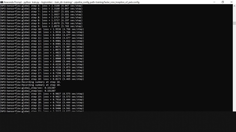
Figure 2. Training of the Model

4. Each step of training reports the loss, which starts high and declines steadily as the training progresses. For example, training on the Faster-RCNN-Inception-V2 model started at about 3.0 and quickly dropped below 0.8. It is recommended to train until the loss consistently falls below 0.05; which takes approximately 40,000 steps, or about two hours (depending on CPU and GPU performance).

Note: The loss numbers will vary if a different model is used. MobileNet-SSD starts with a loss of about 20 and should be trained until the loss is consistently under two.

View the progress of the training job by using TensorBoard*.

This step creates a webpage on the local machine at YourPCName:6006 and can be viewed via your web browser. The TensorBoard page provides information and graphs that show how the training is progressing. One important chart is the Loss graph, which shows the overall loss of the classifier over time.

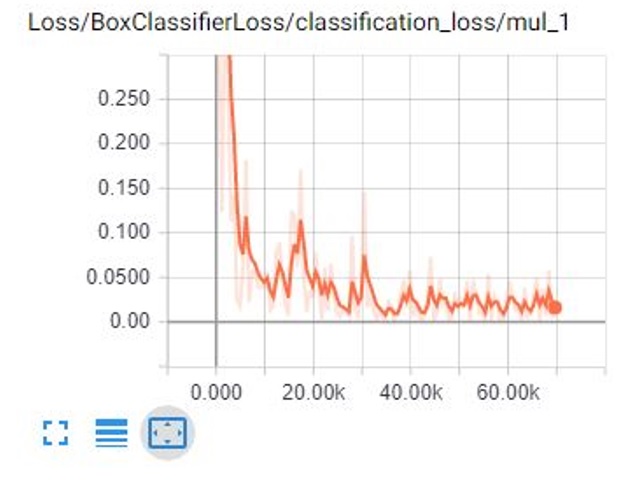
Figure 3. Log-loss graph visualization on TensorBoard*

The training routine saves checkpoints periodically, about every five minutes. To terminate the training, press Ctrl+C while in the command prompt window. Wait until just after a checkpoint has been saved to terminate the training; it can be resumed later, restarting from the last saved checkpoint. The checkpoint at the highest number of steps will be used to generate the frozen inference graph.

5. Now that training is complete, the last step is to generate the frozen inference graph (. pb file) which creates a frozen_inference_graph.pb file in the \object_detection\inference_graph folder. The. pb file contains the object detection classifier.

6. The next focus is on using the Intel Distribution of OpenVINO toolkit to run interfaces. The classifier algorithm helps to identify the plant correctly. First, optimize the model to create an *.xml and *.bin file.

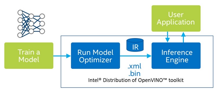
Figure 4. Diagram of the Intel® Distribution of OpenVINO™ toolkit flow

7. Use the mo.py script from the <INSTALL_DIR>/deployment_tools/model_optimizer directory to run the model optimizer and convert the model to the intermediate representation (IR).

Note: Some models require using additional arguments to specify conversion parameters, such as --scale, --scale_values, --mean_values, --mean_file. To learn when to use these parameters, refer to Converting a Model Using General Conversion Parameters.

8. The mo.py script is the universal entry point that can deduce the framework that has produced the input model by a standard extension of the model file:

• .caffemodel - Caffe* models
• .pb - TensorFlow* models
• .params - MXNet* models
• .onnx - ONNX* models
• .nnet - Kaldi* models.

9. Since the model is built on TensorFlow and the frozen inference graph is already generated (. pb file) as mentioned in step 5, use that particular file and run the mo.py script.

10. This approach uses a model optimizer to fine-tune the model for a user application to consume. The .xml and .bin files generated from the model optimizer are consumed by the inference engine using the Python API, which is essentially a wrapper built on top of C++ core codes.

Workflow Steps: Gather Data

When training a robust classifier, the training images should have random objects in the image along with the desired objects, as well as a variety of backgrounds and lighting conditions. In some images, the desired object should be partially obscured, overlapped with something else, or only halfway in the picture. This article uses the package icrawler, which is provided by pypi. For details, go to icrawler pypi.

To install icrawler, run the following command on the Anaconda* prompt:

pip install icrawler

Next, import the icrawler package and write a small snippet of code in Python to fetch the images from Google*.

The command shown below uses a keyword for the web crawler to gather all the results from Google Images* search service and saves them in .jpeg format on the disk. Provide the number of desired images as an input to the code.

from icrawler.builtin import GoogleImageCrawler
for keyword in ['Hibiscus rosa-sinensis', Marigold]:
    google_crawler = GoogleImageCrawler(
        parser_threads=2,
        downloader_threads=4,
        storage={'root_dir': 'images_new/{}'.format(keyword)}
    
    )

Make sure the images are each less than 200KB, and their resolution does not exceed 720x1280. The larger the images, the longer it will take to train the classifier. Use a Python script to reduce the size of the images.

Label Pictures

Here’s the fun part: labeling the desired objects in every picture. LabelImg is a useful tool for this purpose; its GitHub* page has clear instructions on how to install and use it.

1. LabelImg GitHub Documentation
2. LabelImg Download File

Point LabelImg to your \images\train directory, and then draw a box around the object in each image. Repeat the process for all the images in the \images\test directory. This process will take a while.

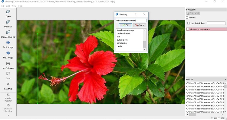
Figure 5. Labeling the objects in an image

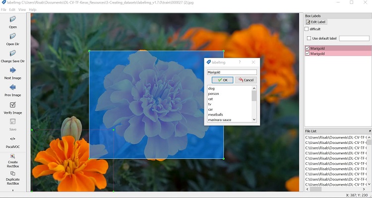
Figure 6. Labeling the object in the image

LabelImg saves an .xml file containing the label data for each image. These .xml files will be used to generate TensorFlow records, which are among the inputs to the TensorFlow trainer. As each image is labeled and saved, there will be one .xml file for each image in the \test and \train directories.

There are 300 images for each species, split for training and testing.

Capture Frames for Processing

For any application that involves the use of image, video, or live camera feed, it is necessary to capture the frames. This process is easy and straightforward to do using OpenCV. Once the frames are captured, iterate through each frame, and pass it through the recognition engine for detection.

To provide an image as an input to the model, use the code described below:

import cv2
IMAGE_NAME = 'test1.jpg'
# Grab path to current working directory
CWD_P # Path to image
PATH_TO_IMAGE = os.path.join(CWD_PATH,IMAGE_NAME)ATH = os.getcwd()
image = cv2.imread(PATH_TO_IMAGE)
image_expanded = np.expand_dims(image, axis=0)

To provide videos as an input to the model, use the following code:

import cv2
cap = cv2.VideoCapture(0)
ret, image_np = cap.read()

To provide live camera feed as an input to the model, use the code below:

import cv2
# Initialize webcam feed
video = cv2.VideoCapture(0)
ret = video.set(3,1280)
ret = video.set(4,720)

The above piece of code captures the video frames. The third line is the one that must be inside a loop as it captures frames.

Plant Recognition Using TensorFlow* Classifier

First, include all the required packages:

# Import packages
import os 
import cv2
import numpy as np
import tensorflow as tf
import sys

# This is needed since the notebook is stored in the object_detection folder.
sys.path.append("..")

# Import utilites
from utils import label_map_util
from utils import visualization_utils as vis_util
# Name of the directory containing the object detection module we're using

MODEL_NAME = 'inference_graph'

# Grab path to current working directory
CWD_PATH = os.getcwd()

# Path to frozen detection graph. pb file, which contains the model that is used
# for object detection.
PATH_TO_CKPT = os.path.join(CWD_PATH,MODEL_NAME,'frozen_inference_graph.pb')

# Path to label map file
PATH_TO_LABELS = os.path.join(CWD_PATH,'training','labelmap.pbtxt')

Include in the classifier code how many classes of plants to recognize. For this experimental research purpose,  we are targeting two plant species: Hibiscus rosa-sinensis and Marigold.

# Number of classes the object detector can identify
NUM_CLASSES = 6

Next, load the TensorFlow model:

# Load the Tensorflow model into memory.
detection_graph = tf.Graph()
with detection_graph.as_default():
    od_graph_def = tf.GraphDef()
    with tf.gfile.GFile(PATH_TO_CKPT, 'rb') as fid:
        serialized_graph = fid.read()
        od_graph_def.ParseFromString(serialized_graph)
        tf.import_graph_def(od_graph_def, name='')

    sess = tf.Session(graph=detection_graph)


# Define input and output tensors (i.e. data) for the object detection classifier

# Input tensor is the image
image_tensor = detection_graph.get_tensor_by_name('image_tensor:0')

# Output tensors are the detection boxes, scores, and classes
# Each box represents a part of the image where a particular object was detected
detection_boxes = detection_graph.get_tensor_by_name('detection_boxes:0')

# Each score represents level of confidence for each of the objects.
# The score is shown on the result image, together with the class label.
detection_scores = detection_graph.get_tensor_by_name('detection_scores:0')
detection_classes = detection_graph.get_tensor_by_name('detection_classes:0')

# Number of objects detected
num_detections = detection_graph.get_tensor_by_name('num_detections:0')

Load the input and view the output window initiated by the model:

                  #ser.write(b'3')
# Initialize webcam feed
video = cv2.VideoCapture(0)
ret = video.set(3,1280)
ret = video.set(4,720)

while (True):

    # Acquire frame and expand frame dimensions to have shape: [1, None, None, 3]
    # i.e. a single-column array, where each item in the column has the pixel RGB value
    ret, frame = video.read()
    frame_expanded = np.expand_dims(frame, axis=0)

    # Perform the actual detection by running the model with the image as input
    (boxes, scores, classes, num) = sess.run(
        [detection_boxes, detection_scores, detection_classes, num_detections],
        feed_dict= {image_tensor: frame_expanded})

    # Draw the results of the detection (aka 'visulaize the results')
    vis_util.visualize_boxes_and_labels_on_image_array(
        frame,
        np.squeeze(boxes),
        np.squeeze(classes).astype(np.int32),
        np.squeeze(scores),
        category_index,
        use_normalized_coordinates=True,
        line_thickness=8,
        min_score_thresh=0.60)

    # All the results have been drawn on the frame, so it's time to display it.
    cv2.imshow(Plant Anatomy, frame)

    # Press 'q' to quit
    if cv2.waitKey(1) == ord('q'):
        break

# Clean up
video.release()
cv2.destroyAllWindows()

Sample Images from the Test Run

Observe how the model has classified the plant types:

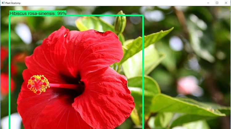
Figure 7. Plant anatomy detection in action

The above image from the test run shows that the model successfully detects the plant. It creates a bounding box and displays the scientific name of the plant species. The above flower is Hibiscus rosa-sinensis and is correctly identified by the model. It also shows the accuracy of detection in percentage; in this case, the recognition accuracy is 99%.

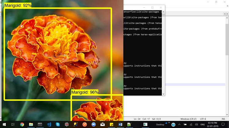
Figure 8. Plant anatomy detection in action

As shown in the above image, the model recognizes the other class of plant species correctly and accurately as well. Moreover, it is evident that if more than one plant is present in the input, it separates them by creating a bounding box. The accuracy of this test case is 92% and 96%.

More Test Cases

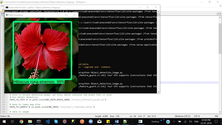
Figure 9. Plant anatomy detection in action

Figure 10. Plant anatomy detection in action

Conclusion

The above illustrates the importance of plant taxonomy in the modern world and how this solution shows accurate results in identifying plant species correctly. The model gives a good use case of deep learning and computer vision; introducing a computer vision recipe using the model optimizer and inference engine of the Intel Distribution of OpenVINO toolkit. The high accuracy rates are due to model optimization. The project is into its next phase, adding more features such as identification of family, class, and genera of the plant species.