This tutorial provides a use case where a credit card company might benefit from machine learning techniques to predict fraudulent transactions. This is the first part of a three-part series.
In this post, you’ll prepare and pre-process data with the Intel® Distribution of Modin*. You’ll also use an anonymized dataset extracted from Kaggle*.
The Intel® Distribution of Modin will help you execute operations faster using the same API as pandas*. The library is fully compatible with the pandas API. OmniSci* powers the backend and provides accelerated analytics on Intel® platforms. (Here are installation instructions.)
Note: Modin does not currently support distributed execution for all methods from the pandas API. The remaining unimplemented methods are executed in a mode called “default to pandas.” This allows users to continue using Modin even though their workloads contain functions not yet implemented in Modin.

Official Intel® Distribution of Modin documentation
Section 1 - Pre-process and Initial Data Analysis
The first step is to pre-process the data. After you download and extract the data, you’ll have it in spreadsheet format. That means you’ll work with tabular data where each row is a transaction (example) and each column is a feature (transaction amount, credit limit, age.) In this tutorial you won’t know which represents each feature, since the data has been anonymized for privacy purposes. This example uses supervised learning, meaning the algorithm is trained on a pre-defined set of examples. The examples are labeled with one column called LABEL (FRAUD or NOT FRAUD) (Image 2).
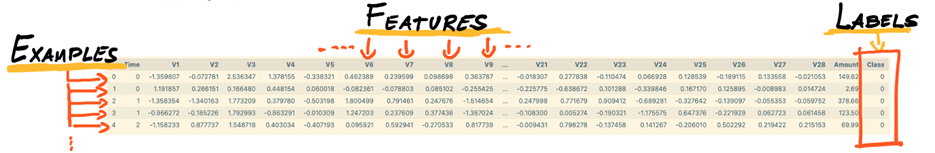
Graphic: Ezequiel Lanza
In a real-world case, the data could come from multiple sources (such as SQL, Oracle Database* or Apache Spark*.) The idea is to have one spreadsheet file to put in the algorithm to train it. To do that, you need to concatenate or join multiple files to get one main dataset. Joining multiple sources can result in a main dataset with thousands of lines and hundreds of columns. Working with such a large file can strain on your computer/server for memory and processing, so it’s important to use optimized frameworks to speed up this task.
First, load the dataset. You’ll use both regular pandas and optimized Modin-Pandas (pd). By using both, you’ll see the difference when your device uses all of its cores instead of using just one core. This will demonstrate how Modin can help.
t0 = time.time()

pandas_df = pandas.read_csv("…creditcard.csv")

pandas_time = time.time()- t0


t1 = time.time()

modin_df = pd.read_csv("…creditcard.csv")

modin_time = time.time() - t1
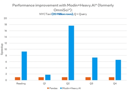
As you can see, the results can be up to 18x faster (Note: Results vary depending on Intel(R) CPU / memory selected + dataset.)
Official Intel® Distribution of Modin documentation
Now that the dataset is loaded on your memory, take a closer look.
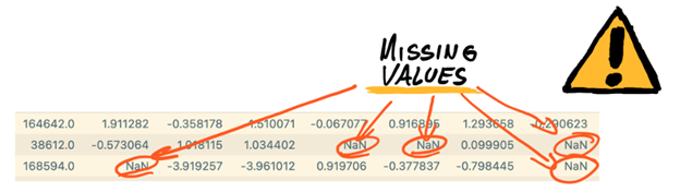
Check for missing values
One of the first steps in data analysis is to check for missing values, because most algorithms can’t handle missing data. This verification is a useful shorthand to see if the data is accurate. It’s important to know how large the problem is to determine how to handle it. For example, 80% missing values is evidence of a bad dataset, but not a problem when that number is closer to 5%.
Graphic: Ezequiel Lanza
There are multiple ways to address this problem. There are no good or bad decisions, try them out and see how the algorithm performs with each.
- Remove the lines with missing values. If there aren’t very many missing values, a smaller dataset won’t be an issue.
- Impute value. Simulate a value to fill in the missing field. The idea is to use the example (line) but reduce the effect of missing values. Try replacing with the mean/maximum/minimum value of the feature (column.) You can also impute based on K-means, which will predict the value with an eye to the other values (columns.)
When you’re working with data extracted from outside sources, it’s worth factoring in system failures. These failures take the form of incomplete reporting – taking only partial snapshots of the dataset – and can result in missing values.
Let's check for missing values:
t0 = time.time()

print(pandas_df.columns[pandas_df.isna().any()])

pandas_time = time.time()- t0


t1 = time.time()

print(modin_df.columns[modin_df.isna().any()])

modin_time = time.time() - t1

Index([], dtype='object')

Index([], dtype='object')
Fortunately, in this example there are no missing values, so you can move on to sub-sampling.
Sub-sampling
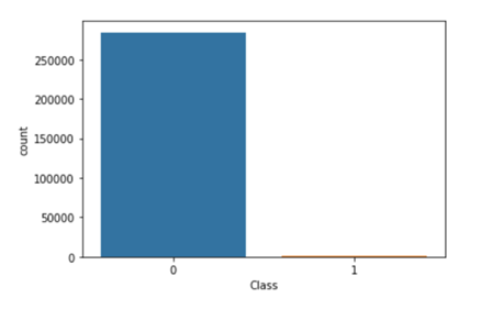
Take a look at the distribution of your data.
sub_sample_plot=sns.countplot(pandas_df["Class"])

sub_sample_plot
Graphic: Ezequiel Lanza
It’s clear that the class (FRAUD or NO FRAUD) is very unbalanced. That means that most cases aren't fraud and just a few are FRAUD.
To train a model with the entire dataset, the model should learn how to detect the majority of cases (NO FRAUD), which is not what we want: We want to detect fraud.
If a model is trained with this data, it would reach high levels of accuracy, but that’s not the outcome you want. (Part three of this tutorial explains how to select a metric based on the criteria you’re seeking.)
Here are some ways to solve this problem:
- Obtain more FRAUD examples. Ask the dataset owner for more examples. Usually, however, you need to work with the dataset you have.
- Increase FRAUD examples: If there are examples of the class you want to detect, use an algorithm to generate a considerable number of examples of the desired class. This solution is used mainly in computer vision scenarios but works for others as well.
- Use a different dataset where the ratio of FRAUD to NO FRAUD is close to 1:1.
Now you’re ready to create a new dataset with a useful ratio for generalizing both classes.
First, create a NEW balanced dataset.
modin_df_sub = modin_df.sample(frac=1)  #Shuffling the dataframe


modin_df_sub_nf = modin_df_sub.loc[modin_df["Class"] == 0][:492]

modin_df_sub_f = modin_df_sub.loc[modin_df["Class"]==1]


# Will reuse all fraud points, will random sample out 492 non-fraud points


# New sample Table

modin_df_sub_distributed = pd.concat([modin_df_sub_nf,modin_df_sub_f])

modin_balanced = modin_df_sub_distributed.sample(frac=1, random_state=42)
The resulting balanced dataset makes it easier to train the algorithm.
sub_sample_plot=sns.countplot(modin_balanced["Class"])

sub_sample_plot
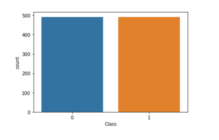
Graphic: Ezequiel Lanza
Conclusion
Now you have the data necessary to demonstrate a fair representation of FRAUD and NO FRAUD examples. It should also be clear what advantages the Intel® Distribution of Modin provides — with no code changes.
In part two, you’ll analyze and transform the data and part three train the algorithm.
Stay tuned!