Abstract
We describe updates to the original conservative morphological anti-aliasing (CMAA) algorithm including a new DirectX* Compute Shader implementation that we call CMAA2. This version provides additional performance, improved quality, optional integration with multi-sample anti-aliasing (MSAA), and the ability to be leveraged asynchronously on graphics processing units (GPUs) that support this capability. We also describe some of the weak points of the post-process anti-aliasing (AA) techniques, reflect on scenarios in which they work well and, in some cases, complement MSAA solutions. In comparison to fast approximate anti-aliasing (FXAA), our testing using the publicly available Amazon Lumberyard* Bistro scene shows that CMAA2 provides as good or better anti-aliasing while preserving significantly more of the input image sharpness at roughly similar performance. At higher resolutions, CMAA2 is as fast or faster depending on the hardware. We provide quality and performance for a number of hardware and resolution configurations as well as the source code to a DirectX* 11 DirectCompute 5.0 sample application.
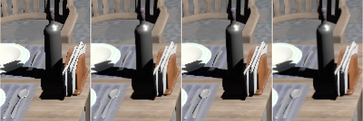
Figure 1. On the left, the image with no anti-aliasing enabled. Second image shows CMAA2 applied alone. Third image is 8xMSAA alone, showing better subpixel AA on the napkin holder and other geometry than the second, but no AA on shadows. On the right is 4xMSAA+CMAA2 providing better AA compared to 8xMSAA alone, at lower overall computation cost.
Introduction
We present an update to the image based conservative morphological anti-aliasing (CMAA) algorithm and discuss the performance and quality tradeoffs as well as the integration with multi-sample anti-aliasing (MSAA). This new implementation improves on the anti-aliasing quality and performance of previous implementations.1 Also, we have transitioned from a pixel shader to a series of compute shaders that can improve performance on hardware that supports the simultaneous execution of work scheduled in a graphics and compute command queue. The compute shaders are DirectX* Compute Shader 5.0 and we provide a sample implementation in DirectX 11. Finally, we discuss how to use CMAA together with MSAA and how the two approaches complement each other.
While we focused on optimizations to improve the performance on Intel® Integrated Native Developer Experience (Intel® INDE) graphics, we worked to ensure the algorithm works well on the latest discrete graphics processing units (GPUs) from other vendors. We welcome contributions from the community to refine the implementation.
The move from a pixel shader to compute shader implementation provided us with several benefits. First, we can schedule the work concurrently on hardware that supports execution of graphics and compute simultaneously via asynchronous compute. Second, we leverage shared local memory which is not available in pixel shaders to avoid more expensive memory access. Third, by leveraging indirect dispatch, we are able to better utilize GPU compute resources when compared to a pure pixel shader implementation, especially for shape detection and resolution which relies on branching in the pixel shader. Many other benefits are described in Section 2 when we describe the improvements over previous releases of CMAA.
For the purposes of this paper, we will use CMAA2 to refer to CMAA 2.0.
Meaning of conservative and morphological
We use the term conservative to refer to the unique approach of classification and resolving of aliasing artifacts designed to preserve overall sharpness of the input image while still providing a visually pleasing aliased result. In other words, our anti-aliasing heuristic is guided by two objectives: getting as close to ground truth as possible while at the same time minimizing the change to the input image. We use the term morphological to identify it as belonging to the same class of algorithms as the original morphological antialiasing.2
Why integrate with Multi-Sample Anti-Aliasing (MSAA)?
Inspired by the work to integrate SMAA with 2xMSAA (SMAA S2x)3, there are a few specific reasons we wanted to investigate the integration of CMAA with MSAA. First, MSAA alone is intended to resolve rasterization artifacts but does not help with aliasing issues that arise during pixel shading, so increasing the sample count above 4x or 8x provides diminishing returns at the exponential increase in cost. Examples of aliasing sources that do not benefit from MSAA are high power specular components, sharp shadow maps or even ray-traced shadows as shown in John Story's "Hybrid Ray-Traced Shadows".4 Second, because MSAA is not as efficient on some integrated GPUs as we would like, higher sample counts can be impractically expensive in certain scenarios. We are able to show that the integration of CMAA2 and MSAA provides a net benefit over doing one or the other individually, providing an effect that is better than the sum of its parts. Specifically, we show that 4x MSAA with CMAA2 can provides higher quality than 8x MSAA at a lower or similar overall performance cost depending on the graphics hardware and share these results in Section 6.
Previous Work in Post-Process Anti-Aliasing
Anti-aliasing techniques have been studied by computer graphicists for many years. For the purposes of this article we limit references to popular post-processing techniques, all of which attempt to approximate a super sampled anti-aliased (SSAA) image taking into account only the pixels generated in the target frame buffer at frame buffer resolution. In some cases which include temporal sampling, SMAA T2x for example, they additionally leverage previously generated frame buffers. Integrated temporal sampling with an earlier CMAA2 implementation is presented in Sungye Kim's "Temporally Stable Conservative Morphological Anti-Aliasing" article.5
A retrospective of the post-processing era is available, so we refer the reader to this survey for more background as well as a survey of games that have shipped that adopted implementations of post process anti-aliasing techniques.6 This has been an active area of work and we will review four of the interesting implementations. First, we will describe morphological anti-aliasing (MLAA) which forms the foundation of our technique as well as the others. Next, we review fast-approximate anti-aliasing (FXAA) which has been widely adopted as a very fast post-process anti-aliasing technique. We also review subpixel morphological anti-aliasing (SMAA) which was used in CRYENGINE* as well as many other titles.7 Finally, we compare our updates to the previous implementations of CMAA.
Post-processing methods
Morphological Anti-Aliasing (MLAA)
A seminal work in the field of post process anti-aliasing is Alexander Reshetov's MLAA paper.2 MLAA was originally implemented as a CPU-side post-processing technique well suited but not limited to ray tracing. Shortly after this invention the technique was implemented on the GPU.8 In Reshetov's implementation, edges in color space were classified as Z, U, or L shapes where Z and U shapes can be decomposed into 2 L-shapes, as seen in the figure below. While we provide a short summary here, it is recommended for those interested in additional details to consult the original paper.
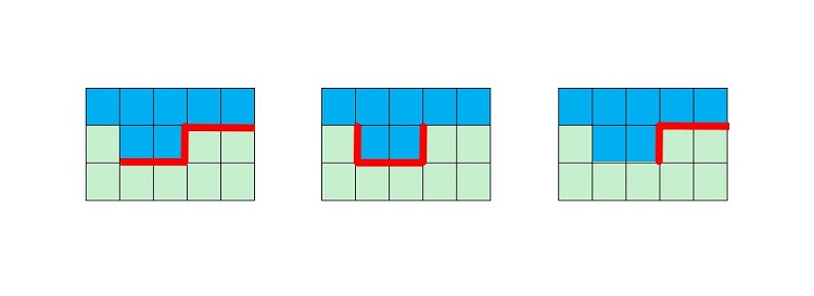
Figure 2. Shapes classified in the original MLAA paper. From left to right: Z, U, and L shapes. The shapes are also identified that match these patterns rotated 90, 180 and 270 degrees. Since Z and U shapes decompose into L-shapes, the MLAA implementation need only be concerned with processing the decomposed version of Z and U into two L-shaped subcomponents.
All of the L-shapes are blended in the final stage by blending the colors of the pixels that touch the edges they contain. To do this blending a primary and secondary edge is defined, the primary edge being the one that was found at the first step, and the secondary edge the one found in the second merge phase. Interestingly, the secondary edge is only one pixel in length, even in cases when the number of pixels detected in a previous phase belonging to the secondary edge could be longer. This is safe because the rest of the pixels not processed in this stage will be independently processed as a separate shape. The pixels are blended based on a weighted average of the area of each pixel occupied, found by drawing a line from the midpoint of the secondary edge to the farthest vertex of the primary edge.
Fast Approximate Anti-aliasing (FXAA)
Like other post-processing techniques, FXAA infers edges in color space and operates only on those edges to minimize the amount of computation. The value proposition of existing FXAA implementations is as follows:
- Executes on the GPU and can vary the performance and quality tradeoffs by adjusting parameters as well as the number of taps used to filter.9,10
- Ease of integration into today's rendering engines
- Improvement in perceived image quality for a minimal sacrifice in frame rate
FXAA has remained a popular and practical post-processing technique, particularly in deferred rendering. The implementation described in FXAA by Timothy Lottes9 is a single pass on the color image and integrates the ability to estimate luminance strictly from the red and green channels observing that blue aliasing rarely occurs in game content. The computations described in "Filtering Approaches for Real-Time Anti-Aliasing",10 are kept localized to the nearest neighbor pixels and optionally increasing the filter width up to 8 pixels. We use a publicly available implementation.11 We use FXAA version 3.11 at default settings for testing and comparison purposes.
Subpixel Morphological Antialiasing (SMAA)
SMAA is an evolution of the original MLAA12 and describes how to handle many issues not addressed in previously published post-processing techniques including local contrast adaptation (LCA), improves handling of sharp corners, diagonal line segments, subpixel features, motion, and specular aliasing. SMAA highlights its modularity allowing the implementation to adapt to discrete design points in quality and performance. For example, a low-end hardware target may choose to include the features to resolve diagonal line segments and local contrast but may omit the temporal stages. Similarly, a high-end target may include all of the capabilities and show even better results in both performance and quality than a high bandwidth MSAA implementation. We use a publicly available SMAA implementation at default settings for testing and comparison purposes3.
CMAA2 and improvements over previous CMAA implementations
Intel has published earlier implementations of CMAA.1 This was a pixel shader-based implementation that had commercial use in game titles, for example CodeMaster* GRID 2.13 We improve upon this previous implementation that we describe in more detail.
- The shape detection heuristics are improved based on parameters that provide a solution closer to the ground truth image tested on a realistic standalone workload as well as a number of image captures from popular 3D content, while further minimizing changes to high frequency texture or areas containing text.
- We minimize the use of memory bandwidth to allow good performance scaling to high resolution render targets. For example, the input/output image is modified in-place and only in areas that require anti-aliasing to avoid the full-screen copy operation common in pixel shader implementations. Also, we leverage shared local memory for intermediary data storage where possible while using efficient encoding for any intermediary data stored in RAM.
- We implement the algorithm with compute shaders to take advantage of asynchronous compute when available.
- We process 2x2 pixel tiles at a time which allows us to launch fewer total threads with more work per thread. This allows us to reduce the memory fetches because samples are re-used for multiple pixels. In addition, the edge detection results can be re-used for the pixels that make up the tile.
- We support the integration of CMAA2 with MSAA.
- We leverage indirect execution on the GPU via the
DirectX DispatchIndirect()method to reduce the amount of work relative to a pixel shader approach that may have required less efficient branching or stencil masking.14 - We support log-luma based edge detection and high dynamic range (HDR) color buffer anti-aliasing.
- The new implementation resolves a race condition in previous versions that could result in sparkling even when the camera was not moving when blending overlapping horizontal and vertical shapes.
TSCMAA 1.0
Intel published a temporally stable adaptation of a recent implementation which enhances the frame to frame coherence of the original CMAA implementation, temporally stable conservative morphological anti-aliasing (TSCMAA).5 In fact, the request for updating the original CMAA for use in the TSCMAA implementation is what inspired this stand-alone CMAA2 update. Given the significant changes, we felt details of the revised CMAA technique independently justified its own treatment, in addition to updates that have occurred since the original TSCMAA implementation.
|
Input |
Detect Edges Locate edges in input images, store as candidates for later evaluation |
→ |
|
Edge |
Process Edges For each edge, calculate new weighted color values, append results to per pixel linked list |
→ |
|
Buffer of per |
Resolve For each pixel of the output image, blend linked lists elements in a weighted average into the output buffer |
|
| Output image |
An overview of the three primary stages of the CMAA 2.0 algorithm. Each stage is an independent compute shader and takes input from the previous stages to compute the final render target. Details of each stage are described below.
CMAA2 Overview
In this section we provide an overview of our CMAA2 algorithm. We compare and contrast with two of the most popular post-process anti-aliasing solutions on the market today, FXAA and SMAA.
High level overview – finding and handling shapes
One way to distinguish different post process anti-aliasing techniques is by looking at the aliasing shapes they identify and how they utilize those shapes to anti-alias by blending with neighboring pixels. Summarizing from Reshetov and Jimenez's presentation6, we can simplify the key points of MLAA or SMAA as follows:
- Finding axis-aligned lines (edges) separating pixel with different colors
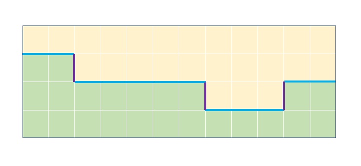
Figure 4. The MLAA edge detection step. - Reconstructing silhouette lines connecting pixels adjacent to both horizontal and vertical separation lines while resolving ambiguity in favor of the longer shape silhouettes and taking into account the resulting shapes
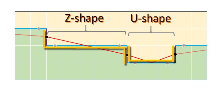
Figure 5. The MLAA shape classification and revectorization step. - For each pixel intersected by the silhouette lines, its color is blended with the color of the pixel on the opposite side of the separation line with weights proportional to the trapezoid areas
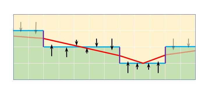
Figure 6. The final MLAA blending step.
CMAA2 uses a first step that is analogous to the first step above (Figure 4), where axis-aligned lines separating pixel with different colors (edges) are found.
However, the fundamental difference from MLAA (and SMAA) is in the rules governing shape classification that follow the reconstruction of the silhouette lines. Here CMAA2 classifies only one main shape type – a symmetrical Z shape, different from the Z, U and L shapes from MLAA and SMAA.
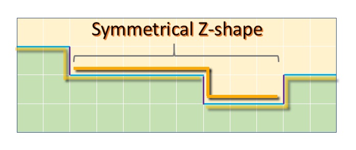
Figure 7. An example of a CMAA2's symmetrical Z-shape.
CMAA2's Z-shape transition from one row or column to the next is always one pixel in height and width, while the arms are extending as long as it can walk an unbroken color edge on the sides, with the additional constraints that the length of one arm is never larger than the length of the other multiplied by a constant value, for example 1.2, 1.3, or 2, and they always have a combined length of at least 4 pixels.
Finally, the blending is performed assuming the underlying geometry's silhouette is a straight line from one to the other Z-shape arm's centers.
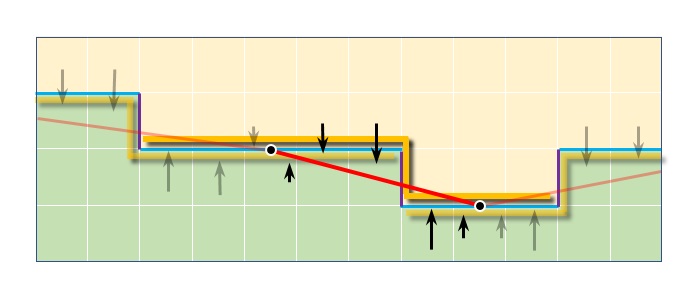
Figure 8. The revectorization (red line) and blending based on CMAA2's symmetrical Z-shapes. The blend takes place between the midpoint of the two long arms of the z-shape.
This symmetrical Z-shape classification and blending approach is the core of the CMAA2 approach and is more restrictive when compared to the one employed by MLAA (and consequently SMAA). Symmetrical Z handling inherently avoids the over blurring scenarios that are handled as a special case in SMAA using the longer crossing edges condition, as described in Chapter 4.2 Pattern Handling – Sharp geometric features12.
Figure 9. From left to right: the source image, FXAA 3.11, SMAA, and CMAA2.
Figure 9 shows different behaviors of FXAA, SMAA and CMAA2 on a simple synthetic example of a simple rotating square, with visible differences in sharpness and handling of corners. Next, we will cover the practical implications of these differences in the real-world scenarios.
CMAA2's simple shapes
A careful observer will notice that there is one-pixel blurring in the corners of the CMAA2 case and also that we have previously stated that one of the conditions for the detection of a symmetrical Z-shape is that "the combined length of the arms is 4 or above”. This would have excluded these corners as well as a subset of other aliasing artifacts such as a diagonal line.
CMAA2 uses a separate simple shape detection and filter to handle these cases. This simple shape filter works on pixels individually, taking as input info on the 12 surrounding edges as shown in Figure 10 and performs re-vectorization and blending between the pixel and its four neighbors (left, top, right, bottom). The blending weights computation is based on a relatively simple heuristic that is explained in the implementation details. This filter is not executed on pixels that were previously processed by the main symmetrical Z-shape.
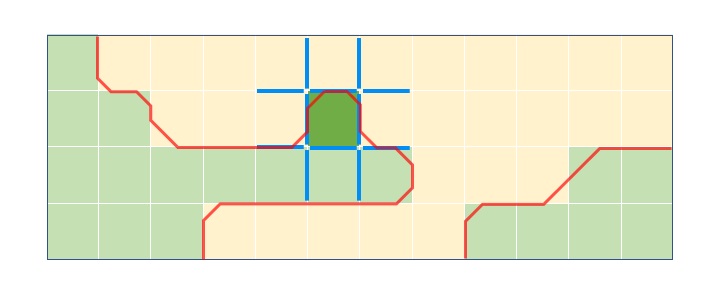
Figure 10. CMAA2's handling of secondary 'simple shapes'. The blue lines indicate 12 edges used to resolve blending for the dark green pixel in the center and red lines indicate resulting revectorization.
Additional differences from SMAA
CMAA2 does not yet include advanced handling of diagonal aliasing patterns such as the SMAA approach based on using precomputed texture to obtain more accurate coverage areas (Chapter 4.2 Pattern Handling – Diagonal patterns, 11). This is because our implementation of this approach had a non-trivial impact on performance and also reduced sharpness in certain scenarios, which goes against the conservativeness ethos. However, we are still exploring potential solutions, as this is one area where SMAA produces superior quality results compared to both FXAA and CMAA2.
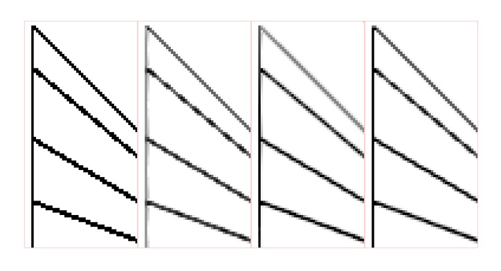
Figure 11. Handling of diagonals, from left: source image, FXAA 3.11, SMAA, CMAA2
CMAA2 extra sharpness mode
There are a number of places throughout the implementation where a tradeoff is made between preserving the sharpness or applying more anti-aliasing. For example, the strength of local contrast adaptation for edge detection, processing symmetrical Z-shape constraints, simple shape re-vectorization aggressiveness, etc. We have captured these settings under a global "Extra sharpness" switch, providing the user an easy way to toggle between two modes. In some scenarios, such as when text and the UI are embedded into the 3D scene, or the art contains sharp high frequency textures, extra sharpness is desirable. In others, more anti-aliasing provides more pleasing results.
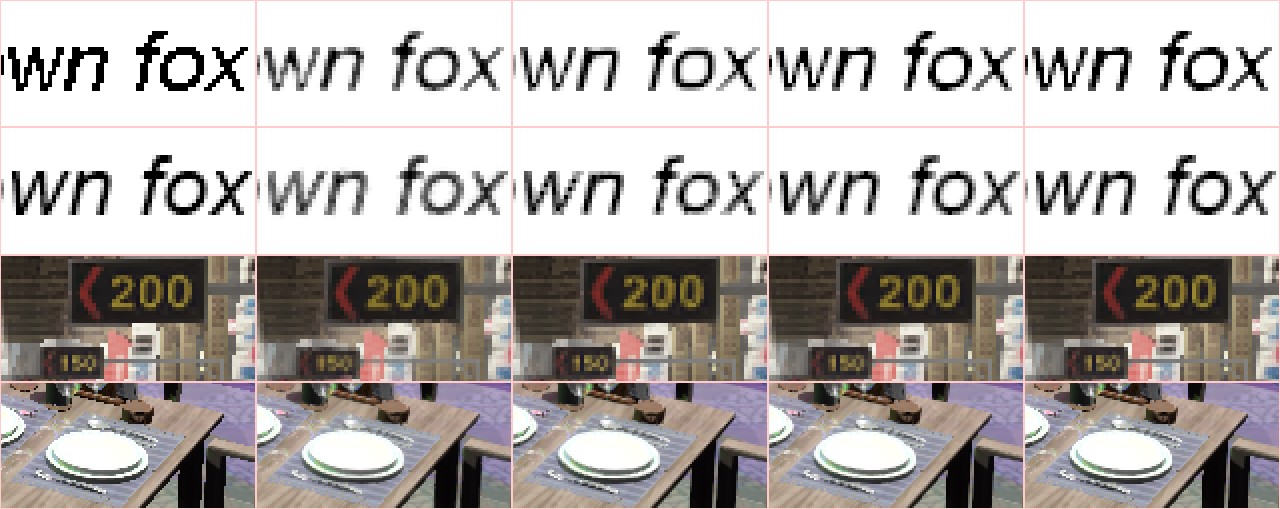
Figure 12. Sharpness vs anti-aliasing; from left: source image, FXAA 3.11, SMAA, CMAA2, CMAA2-ExtraSharpness
Implementation overview
The CMAA2 algorithm is broken into three phases: Edge Detection, Shape Processing, and Resolve. To simplify the process of understanding the overall algorithm we will provide an overview then describe the enhancements to the basic algorithm separately:
- Edge Detection: On an input image, determine edges by examining the color change between a pixel and its neighbors to the north, south, east, and west. If above a threshold, encode this into an edge texture as a simple binary value (Yes = 1, No = 0) in each direction where we use the R,G,B,A channels to represent east, south, west, and north respectively, and append to the shape candidate pixels the (x,y) from the input image into a buffer to be evaluated in the next pass. The shape candidate pixels are a subset of pixels that qualify as either a potential simple shape or a potential complex shape (center of a symmetrical Z-shape) which need to be evaluated in the next phase. At this point no color blending has taken place, only outputs are edges and candidate pixels.
- Shape Processing: Working from the shape candidate pixels and edge information identified in step 1, we determine if we are handling a simple or complex shape. If it is a simple shape we calculate a weighted average of this pixel and its neighbor(s) and store this result into a deferred pixel list as an (x,y) input image position and the new color value. If we also identify it as a potential complex shape using a slightly more complex heuristic than in step 1, we perform full Z-shape measurement by walking the edge on both sides, and if the required constraints are met we perform neighbor blending and store the result in the same deferred pixel list as the simple shapes. Since each pixel may be the member of more than one shape we will later need to blend the color results from all of the shapes it has membership. To this end, we create a linked list and append new pixel values to this linked list as they are calculated. As each pixel in the shape is written out we add this node to the linked list of deferred color values and update the head pointer to this new head node as well as update the head node for this linked list. We call these deferred color values because we have deferred writing the final output pixels to the next stage.
- Resolve: After step 2, we have a set of blended color values for each pixel that need to be merged into the final render target. For each pixel we traverse the values and blend the per pixel results using a weighted average. We weight complex shapes more heavily than simple shapes because the former anti-aliasing heuristic is more accurate and takes precedence while the latter fills in the gaps. This one final color is then written out to the output buffer, and the value is not affected by the order in which the shapes are processed. This decoupling of shape processing and final blending is why we refer to this last step as a deferred resolve.
Implementation Details
Now that we've presented an overview of CMAA2, we present the enhancements and next level of detail on our implementation. First, we describe several improvements made to the base algorithm, including the use of dispatch indirect and optimizations to increase utilization of data we had pulled from memory into the cache and registers. In addition, we describe our encoding scheme for internal data structures and the use of shared local memory, as well as interoperability with MSAA. The next section goes into detail on each of the three phases of the implementation. To motivate these optimizations, it is useful to be familiar with the Compute Architecture of the Intel® Integrated Development Environment graphics GPUs. An excellent reference is the whitepaper, The Compute Architecture of Intel® Processor Graphics Gen9. Also, we assume the reader is familiar with terms related to the DirectX API such as groupshared, dispatch indirect, and threadgroup.
CMAA2 enhancements
Section 3 provided an overview of the CMAA2 algorithm and we continue to instill improvements. However, we continue to evolve the implementation with improvements. To this end, we will describe several of the enhancements included in this version. Also, the Compute Shader Model 5.0 implementation has been tested and is designed to work in both DirectX11 and DirectX12.
Leverage of dispatch indirect
For the second (Shape Processing) and third (Resolve) stages we utilize dispatch indirect to efficiently coalesce and schedule useful work that results from the previous stage and avoid processing pixels that do not require anti-aliasing. This way we can also split the work in 14 optimal thread group sizes that are tuned with regard to shader shared local memory, known as [groupshared] in DirectX High-Level Shading Language (HLSL) and minimize register pressure. For setting up the dispatch indirect calls we invoke two trivial Compute Dispatch Argument passes, omitted in the previous description for clarity, before the second and third main steps. This is in contrast to our original pixel shader CMAA implementation (and SMAA as well) which rely on stencil masking to avoid unnecessary work in subsequent passes on areas that do not require anti-aliasing. Using the stencil mask for this is less efficient than the dispatch indirect approach because of the need and cost of outputting and later using the stencil mask as well as pixel shader thread dispatch granularity that results in some maskedout pixels with no required work still causing the dispatch of redundant threads
Processing source color in 2x2 micro tiles
During performance analysis we observed that the first compute shader version that processed a single pixel per thread was underutilizing the hardware threads on the Intel® Integrated Development Environment graphics GPU as well as performing sampling and math operations where the results could be shared with neighboring pixels. After some experimentation we determined that processing pixels in 2x2 micro tiles per thread provided the right balance between the front end launching thread groups and the back end, as well as the reuse of texture sampling, edge and local contrast adaptation computation. The downside of coalescing the work of four pixels into a single thread is that it increases the complexity of the first stage but in the end the speedup was worth it. These benefits translate directly to discrete GPUs which had similar underutilization issues.
Efficient run-time encoding of data throughout the implementation
In edge detection, we encode the edge candidates into a 4-bit per-pixel buffer using the bits as on or off flags to indicate presence of an edge in each direction. This means that each 2x2 pixel block writes only 16 bits of edge information, which significantly reduces overall memory bandwidth usage of the algorithm.
For intermediate storage of 8-bit non-HDR sRGB packed colors we adopt the R11G11B10_E4_FLOAT encoding from the Microsoft DirectX* 12 MiniEngine, and for processing of HDR color we support standard R11G11B10_FLOAT encoding. It is trivial to extend this to any other encoding if needed although using an encoding that requires more than 32-bits per color will increase memory bandwidth usage and storage requirements. An analysis of small float format precision for storing and using color information can be found in Bart Wronski's "Small float formats – R11G11B10F precision".16
Tight packing of data is employed in all other cases such as when storing the blending values created in Process Shapes and consumed by Resolve. All of these routines are documented with source provided in the sample code and will work on MSAA or non-MSAA surfaces with no changes.
Make use of shared local memory during edge detection
We pack edge information into shared local memory (in HLSL) during edge detection. This provides speedup compared to global memory because we can take advantage of the heavily banked shared local memory portion of the L3 cache on Intel® Integrated Development Environment GPUs. Discrete GPUs also benefit from this optimization.
Make use of shared local memory for coalescing work within a single shader pass
One issue we face in the shape processing pass is that only a small subset of candidates will produce viable Z-shapes, and the processing of each is comparatively an expensive operation. This is problematic as most of the threads in the threadgroup used for evaluation will not result in viable Z-shapes and will continue idling while they wait for the few threads that did find viable Z-shapes to finish their lengthy and expensive operation that involves texture reads, blending and storage operations. In order to reduce the resulting underutilization of the hardware threads we measure the viable Z-shapes as before but then split further blending and processing operations into individual per-pixel micro work items, with arguments encoded into SLM memory. Then, after a group barrier and group sync, we redistribute these work items to all threads in the group and execute them in parallel. Please refer to CMAA2_COLLECT_EXPAND_BLEND_ITEMS macro in the source code for more details.
Interoperability with MSAA
One can attempt to apply post-process AA after the MSAA resolve but this breaks down for areas already anti-aliased with MSAA since edge detection and heuristics no longer have the original values and cannot correctly deduce rasterization artifacts.
More advanced integration of post-process AA with MSAA is explored in detail in SMAA11 for the SMAA+2xMSAA mode called SMAA S2x, where applying the effect on a per-sample-plane before MSAA resolve is shown to induce unwanted blurring. This happens because rasterization for each MSAA sample plane is effectively offset in order to extract subpixel information, so the assumptions on underlying geometry that the post-process AA techniques will make based on the produced image will be shifted and result in divergence from actual geometry, with noticeable blurring. To remedy this, SMAA S2x uses specialized offsetted revectorization heuristics based on the MSAA sample plane offset, as described in11 chapter 4.3 Subpixel Rendering, which counters the rasterization blurring and produces sharp geometry anti-aliasing. However, it does introduce additional blurring on non-rasterization aliasing artifacts that come out of pixel shading because during MSAA pixel shading is done per-pixel and at pixel centers without offsets so in this case the heuristic actually causes a reduction in sharpness.
Initially we tried to separate rasterization aliasing artifacts from pixel shading aliasing artifacts in the MSAA surface by assuming the former on pixels with different sample values within a pixel and later when the MSAA samples within the pixel are identical. This proved to be a relatively good heuristic with regards to quality, but the complexity did not allow for performance that was practical.
Consequently, we decided to revert to the simple CMAA2 + MSAA per-sample-plane approach, with an optional reduction in the CMAA2 effect strength to reduce blurring. Interestingly, although the slight increase in blurriness is noticeable, we still get good quality results that get closer to the ground truth reference (see the section in Chapter 5: CMAA2 Integration with MSAA) in 2x, 4x and 8x MSAA scenarios, and in the case of CMAA2+4xMSAA better quality than 8xMSAA alone. This is potentially due to higher overall sharpness and more conservative revectorization employed by CMAA2 in general when compared to SMAA. From performance perspective, avoiding the offsetted revectorization lets us handle identical samples as one, resulting in acceptable overall cost.
However, we would like to stress that the integration of the CMAA2 and MSAA is provided as a reference, and we have a number of potential future optimizations not yet explored.
Support for edge detection in a previously computed log-luma texture
Edge detection can optionally be supported in an 8-bit per-pixel (bpp) pre-computed log-luma texture to reduce memory bandwidth in the first pass by a factor of four at the cost of slightly lower quality edge detection. This is most useful when previous stages may have already generated such an image and we are able to re-use the texture.
Phase 1 of 3: Edge detection
Edge detection operates on blocks of pixel data with user configurable size, each outputting edge data and anti-aliasing shape candidates. It is contained entirely in the EdgesColor2x2CS function in the provided shader source code. We empirically found that the optimal processing block size on all tested hardware is 32x32 pixels. This results in effective processing of 28x28 pixels by each block since the 2-wide borders of the kernel are used to provide neighbor data to the inner kernel but cannot produce valid output themselves.
What is the algorithm to detect edges?
Edge detection is done in sRGB (not linear) color space to better detect edges that the human visual system is more likely to observe in a scene. For each pixel, we use the pixel to the right and bottom to determine if the color difference is above a threshold and if so we consider it a candidate edge to be evaluated later. A lower threshold will cover more aliasing cases but increase the overall execution time as this results in more edges being considered to require filtering. This difference is measured as the maximum difference in color channels between a pixel to the right and bottom of the current pixel under consideration. In a higher performance implementation, we only measure the difference between precomputed luma values. We store these differences in shared local memory (in DirectX) for later processing.
RGB vs. Luminance in Edge Detection
Edge detection is done using the RGB values to create a luma approximation [Wiki 2018]. We experimented with using RGB directly; however, luminance proved to be faster with minimal quality loss. As an alternative to the supplied RGB to luma based approximation scheme we also include an optional edge detection using a luminance map that may have been created for other stages in the rendering pipeline, for example a tone mapping post process. We leave it up to the user to decide what works best in their specific use case.
Euclidean Distance Metric
The sample code also includes an optional weighted euclidean distance metric for higher quality edge detection. Our experimentation did not show significant improvement in quality that justifies the added performance cost.
Local Contrast Adaptation
To avoid smaller color discontinuities being considered with the same importance as the more noticeable ones, in the second part of edge candidate detection we apply a local contrast adaptation (LCA) step that culls edges when a lot of higher contrast ones exist in the neighborhood. In a technique similar to SMAA as described in Chapter 4.1 Edge detection – Local contrast adaptation11 we reduce the already computed color or luma difference by the maximum of the four values representing connecting edges of opposite orientation, multiplied by a user-selectable contrast adaptation multiplier as in Figure 13. For more detail refer to the ComputeLocalContrastV and ComputeLocalContrastH functions in the shader code. We use shared local memory to keep this computation entirely in GPU memory.
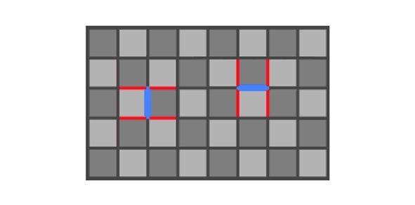
Figure 13. Local contrast adaptation suppresses the blue edge value by the four connecting red edge values of opposite orientation.
Finally, if the remaining value is above the threshold, the edge is considered to be present and we store this as a binary flag for the edge.
Outputs
The last part of the edge detection phase has two parts. One is to coalesce the edge information so that each pixel's processing location holds a full set of flag values indicating the presence of an edge towards each neighbor. This 4-bit value is stored in a 2D texture that we call the edges working buffer. In the second part, this information is used to identify if the location can be a starting point for a simple or complex aliasing shape and if that is the case it is stored in a global list that we call shape candidate list for later processing.
Phase 2 of 3: Processing candidate edges
In the second phase we process the locations identified in Phase 1 and stored the results in the shape candidate list. We spawn one instance of ProcessCandidatesCS per shape candidate using an indirect dispatch on the GPU18 and process each using the following steps:
- For each location, we obtain results of the edge detection for this location and the four neighboring locations by reading from the edges working buffer.
- We then perform simple shape classification and computation of blend values based on the previously obtained edge information – specifically, we use the four edges between the pixel and the neighbors and the additional connecting 8 edges as shown in Figure 14. For more detail refer to the ComputeSimpleShapeBlendValues function in the shader code.
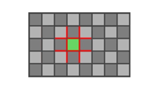
Figure 14. Simple shape kernel size; 12 edges used for shape classification shown in redIf the resulting classification from Step 2 requires color blending, it is performed between the pixel and its four neighbors and the final color value is stored in a separate list using the StoreColorSample function in the shader code, for processing in the last phase.
- Next, after dealing with the simple shapes, we determine whether this can be a starting location for the complex shape, also known as a symmetrical Z-shape, shown previously in Figure 7. We compute the base fitness score of the location for starting the Z-shape for each of the four 90-degree orientations using the DetectZsHorizontal function in the shader code, with the vertical two cases done using the same function just with rotated inputs. The scoring algorithm is based on heuristics that use already loaded edge information as the inputs and is designed to enable early exit before the next step. It is also designed to discern between starting points that are more likely to be a valid triangle rasterization step or that could be part of the texture, text or similar. In the current implementation we pick the Z-shape with the highest score, which also means that we only consider one from a single location even though it possible to consider more. We did this because quality benefits of considering more than one are minimal but the performance considerations are significant.
- If the Z-shape fitness score from the previous step is zero or below, we can exit the thread. Otherwise, we measure the length of the entire Z-shape by tracing the unbroken edge on each side, stopping if one edge becomes a lot longer than the other with the maximum difference ratio being a user constant, 1.5 by default. This is illustrated in Figure 15 where points Ls and Rs indicate locations of the trace start while Le and Re indicates where it ended. In this example tracing on the left stopped when the edge became broken, while tracing on the right ended because the length of the traced line on the right (13 pixels) became 1.5x of the length on the left (9 pixels). Final lengths are then reduced by the fitness score from the previous step which helps preserve sharpness as we found out empirically.
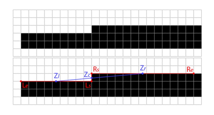
Figure 15. Tracing the edges to determine Z-shape arm lengths - If the combined length of the traced Z-shape arms from the previous step is less than the constant value that is currently set to 5.0, we consider the shape not suitable and exit. Otherwise, we proceed with the assumption that the edge of the underlying geometry spans between the geometric centers of the traced lines (centers of the Z-shape arms), Zl = 0.5 * (Ls + Le) and Zr = 0.5 * (Rs + Re) as illustrated in Figure 16.
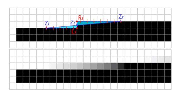
Figure 16. Applying anti-aliasing based on the Z-shapeWe then observe the area that the assumed geometry edge covers for each pixel so we can determine the amount of under-representation: Zl, Zc and Ls define the triangle on the left side of the Z-shape that is under-represented and equally Zr, Zc and Rs define the triangle on the right. We then attempt to correct the under-representation by assuming that the missing color information is best represented by sampling the values below (left) or above (right) of the traced line and blending the color value of each pixel on a line with it, with the ratio corresponding to the area of the pixel covered by the under-representation triangle. This process (shown as red arrows in Figure 16) accounts for most of the anti-aliasing effect in CMAA2. We store the color values from the previous step in the same way we stored color values from processing the simple shapes, by using the StoreColorSample function with an additional flag to indicate that the values are coming from the complex shapes (Z-shapes), so the last stage can distinguish between the two.
Phase 3 of 3: Resolve
The previous stages used the StoreColorSample function to write the anti-aliased color values they expected to store into the final input/output color buffer. Considering that output pixel locations of these color values can sometimes overlap between different complex shapes and between simple shapes and complex shapes, and the processing happens in parallel on the GPU in a non-deterministic order, we store them in separate per-pixel lists and process them together to ensure determinism. Final color value for each pixel is computed as a weighted average with the values originating from complex shapes processing having 10x the weight compared to those from the simple shapes which is a simple way to ensure that the former, higher quality heuristic has the priority. At the end, the final color values are written to the input/output color buffer.
Interoperability with CMAA2 and MSAA details
One major upgrade for CMAA2 is its interoperability with MSAA. An obvious approach would be to simply apply one pass after the other. While this would correctly solve most non-rasterization sources of aliasing since these are not affected by MSAA, it would not do a good job in areas already anti-aliased by MSAA since edge detection and the other heuristics are no longer dealing with the original color values. See Figure 17 for an example.
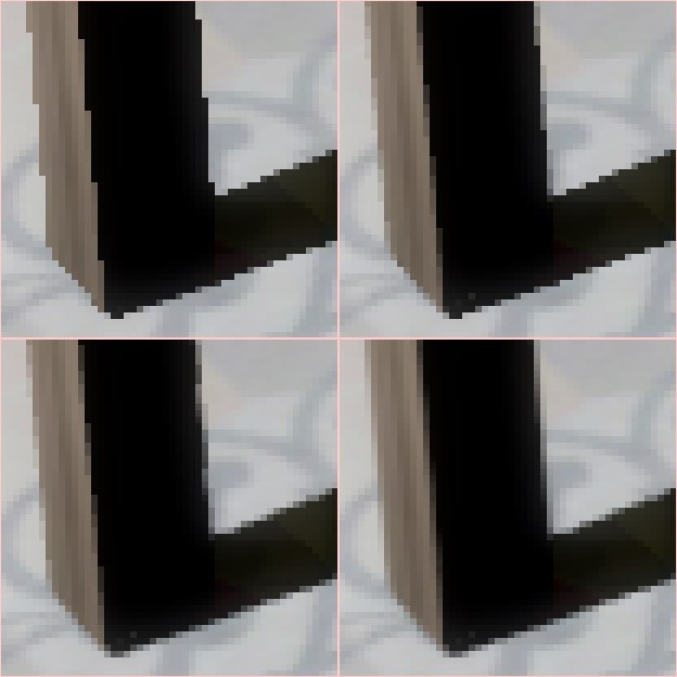
Figure 17. A zoomed in image of a table leg showing geometric and shader-based aliasing. The geometric aliasing is along the leg itself, and the shadow demonstrates the shader-based aliasing. Top-left: no AA; top-right: 4xMSAA; bottom-left: 4xMSAA+CMAA2 applied sequentially (the obvious approach); bottom-right: 4xMSAA+CMAA2 applied per-plane (a more visually correct approach)
Instead of applying the techniques in two separate passes, we instead apply CMAA2 to the individual MSAA planes before the resolve phase, without taking account of individual MSAA sample offsets as explained in Chapter 4: Interoperability with MSAA. This way anti-aliasing of rasterization gradients is enhanced with what we consider an acceptable amount of unwanted blurring and the shading aliasing artifacts are resolved in the same way as they would be with no MSAA, with no additional blurring.
Tone mapping with CMAA2 and MSAA
Another issue to handle with MSAA surfaces is tone mapping which generally applies a non-linear color transform. The result of this is a significant loss of the MSAA effect in high contrast areas when hardware resolve is used. Instead, most modern graphics engines that use MSAA will perform a custom step which resolves MSAA samples after tone mapping [Persson 2008] or perform an inverse luma-weighted blend. In the case of CMAA2 with MSAA, we intercept the custom post-tone mapped resolve to additionally output tone mapped per-sample (not after the multi-sampled resolve) values into a 2D texture array or another multi-sample texture, in addition to regular output for the resolved color buffer. This step can be skipped if tone mapping is not performed. We also create a complexity map texture during tone mapping or separately which is the equivalent of the GL_EXT_shader_samples_identical OpenGL extension20.
Optimization of CMAA2 with MSAA
Instead of trivially applying CMAA2 on each multi-sample (MS) plane separately and then resolving, each of the three CMAA2 compute shader passes are extended to support the processing of MS surfaces, operating on unresolved MS color buffers as the input and the resolved color buffer as the output, using the information from the complexity map to avoid repeating work on identical samples.
The first part of edge detection can skip subsequent loading of the colors, computing and storing the strength values to shared local memory in cases when the texel and its right and bottom neighbors are classified by the complexity map as all having identical samples. This was implemented in the prototype and in our testing has an execution savings of 30-40% for the CMAA2+4xMSAA scenario.
However, there are a number of potential opportunities for future optimization of the CMAA2+MSAA code, such as having API access to the GL_EXT_shader_samples_identical-like information to avoid computing it manually and being able to efficiently apply tone mapping to the unresolved MSAA color texture, both in order to avoid copying values to intermediate texture array, as well as to enable the usage of the more efficient hardware MSAA resolve.
Validation of Edge detection
For improved usability and validation, we implemented a debug draw mode. This allows us to see the edges detected in the Edge Detection phase. This mode was also used in practice to adjust the edge detection threshold and can be enabled by calling DebugDrawEdgesCS after edge detection as shown in the sample code.
Performance and Quality
While ease of integration and suitability to specific scenarios is important, choice of a post-processing anti-aliasing (AA) technique will depend mainly on quality and performance. We provide full DirectX 11 source code for the sample that, in addition to the test 3D scene, has the ability to load any user image and apply CMAA2, FXAA and SMAA in order to test performance and quality, and to find the best settings. We also provide our analysis based on the Amazon Lumberyard Bistro scene, available from the Open Research Content Archive. The interior part of the scene geometry has not been significantly modified, however in order to keep the assets within practical size the textures were downsized and compressed using block-based compression (BC) and some parts of the scene exterior geometry was removed. The reduction of texture resolution reduces the sharpness and detail of the scene to a degree, but the scene remains representative of an average real-time graphics workload, is easily accessible at under 250 MB, and can run on low-end hardware.
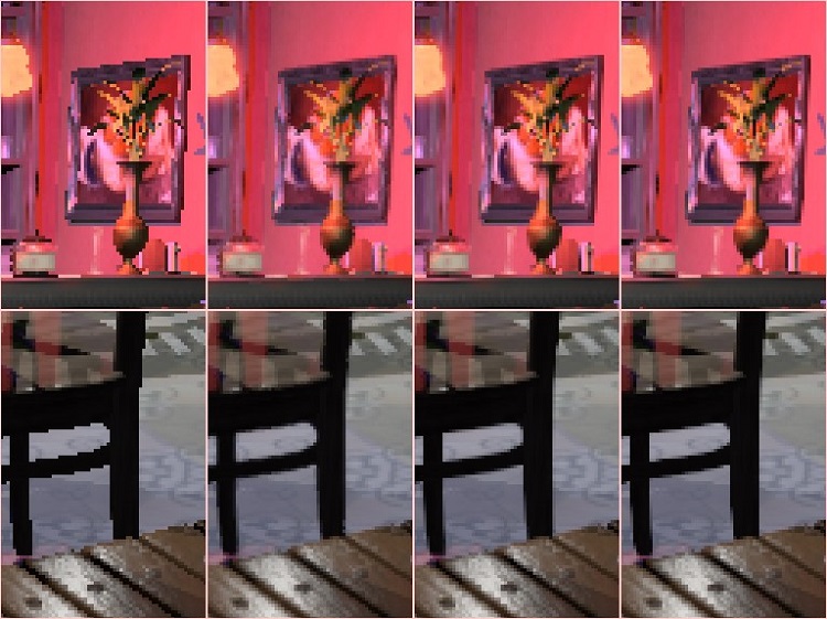
Figure 18. From left to right: Source, FXAA, SMAA and CMAA2.
The FXAA implementation that we use is available at12 and was only modified to consume input luma from a single channel R8 texture using an optimal gather texture sampling codepath. We use default edge threshold and quality settings, with the exception of fxaaQualitySubpix which was adjusted from the default of 0.75 to the value of 0.55 which provides a sharper effect and best peak signal-to-noise-ratio (PSNR) versus ground truth reference numbers, with no change to performance. In the future we plan to also integrate the compute shader FXAA implementation from Microsoft21 as compute shader implementations are more relevant for modern engines.
For SMAA we use the implementation available at GitHub*, upgraded to DirectX 11, at default settings with no changes. We are not aware of a public compute shader implementation but intend to update the code if it becomes available.
Quality
Visual inspection shows that, in general, CMAA2 and SMAA produce a sharp image with some degradation of textures and text, with the exception of a couple of fail cases mostly in the synthetic tests, the difference is minimal. FXAA is blurrier in all scenarios, even with fxaaQualitySubpixreduced at the expense of AA quality. The CMAA2 Extra Sharp mode is clearly best with regards to preserving the input image at the expense of handling fewer aliasing artifacts. With regards to anti-aliasing quality, both CMAA2 and SMAA provide clean, visually pleasing results and SMAA has unrivaled handling of diagonals. FXAA provides smooth anti-aliasing effect with loss of sharpness that can be noticeable in some scenarios and acceptable in others.
For numerical analysis we use the Amazon Lumberyard Bistro scene. We compare image differences to the 8xMSAA reference, to the super-sampled reference and to the raw source images. The super-sampled reference has 36 taps per pixel each at 8x MSAA. The numbers provided below are the average of PSNR differences computed at 8 different test scene locations, at 1920x1080 on Nvidia GeForce* GTX 1070. This may not be fully representative of your title, studio or workload. This is one of the reasons we provide a working implementation that can be used to apply the effects on any input image.
| AA Technique | PSNR (db) Compared to | |
|---|---|---|
| SS Reference | Source (no-AA) | |
| None | 35.28 | None |
| FXAA | 36.75 | FXAA |
| CMAA2 ES | 36.63 | CMAA2 ES |
| CMAA2 | 36.86 | CMAA2 |
| SMAA | 36.67 | SMAA |
| 2xMSAA | 37.85 | 2xMSAA |
Table 1. Various AA techniques, PSNR (db) from SS reference and from source (no-AA).
We can make a couple of observations based on the numbers in Table 1:
- Out of the tested post-process AA approaches CMAA2 is closest to the super sampled reference (36.86), followed closely by FXAA (36.75), SMAA (36.67) and CMAA2 Extra Sharp mode (36.63), with the differences between them being relatively small and context-dependent. As a reference, on the PSNR logarithmic scale these improvement over the no-AA source image (35.28) are roughly around 60% of the improvement that 2xMSAA provides (37.85).
- If we focus on the amount of image change to the source image caused by each approach, we note that the CMAA2 Extra Sharp mode causes the smallest change (42.61), followed by CMAA2 (40.82), SMAA (39.31), and FXAA (37.84).
Our conclusion is that all three techniques provide similar PSNR results when measured as the difference to the super sampled reference, however CMAA2 and CMAA2 Extra Sharp modes achieve this with the least amount of change to the source image, thus preserving most of the detail of the original, while FXAA causes the most significant amount of change (mostly noticeable as unwanted over-blurring).
It should be noted that a smaller PSNR difference from the super sampled reference does not necessarily imply a visually less aliased image. For example, a post-process AA technique can (and will) make incorrect assumptions on the underlying geometry and perform reconstruction that deviates from the ground truth but is still visually pleasing. This can still be a net gain and the balance depends on the input content and visual requirements. This is why we added the Extra Sharp mode – we prefer the way default CMAA2 looks as it has less aliasing than the Extra Sharp mode, but in some cases the latter will be preferred. The same point can be made for SMAA and FXAA; there are cases where SMAA's handling of diagonals and other higher-end features produce better looking results and cases where FXAA's loss of sharpness can be acceptable or even desirable, such as for example with anti-aliasing of ray-traced shadows, as demonstrated in Hybrid Ray-Traced Shadows.4
Performance
We measure performance by timing a deterministic 4800 frame flythrough of the Amazon Lumberyard* Bistro scene, with the performance cost of each AA technique defined as the delta of the full run with it enabled compared to the baseline with no anti-aliasing. This gives an average added performance cost for each technique per frame. We repeat the process and compute an average out of four runs. The test can be performed with the "Run performance benchmarks" option in the code sample 1.
| Added Performance Cost of AA Techniques, as Average Over 4800 Frames, Milliseconds | |||||||
|---|---|---|---|---|---|---|---|
|
|
Nvidia GeForce* GTX 1080 | AMD Vega 64 | Intel® NUC Kit NUC8i7HVK | Intel® NUC Kit NUC6i7KYK | |||
| 1920x1080 | 3840x 2160 | 1920x1080 | 3840x 2160 | 1920x1080 | 3840x 2160 | 1920x1080 | |
| FXAA | 0.11 | 0.37 | 0.09 | 0.30 | 0.24 | 0.82 | 0.94 |
| CMAA2 | 0.15 | 0.38 | 0.10 | 0.24 | 0.22 | 0.59 | 0.73 |
| SMAA | 0.30 | 0.98 | 0.23 | 0.80 | 0.64 | 2.12 | 2.20 |
1 Platform Configuration: Nvidia GeForce* GTX 1080: Windows® 10 64-bit Build 16299, Intel® Core™ i7-6950 processor @ 3.0Ghz, 16384MB RAM, Nvidia Geforce GTX 1080, 16221 MB Display Memory, Driver Version 23.31.13.9135, System Manufacturer and Model: MSI MS-7885. AMD Vega 64: Windows 10 64-bit Build 16299, Intel Core i7-6950 processor @ 3.0Ghz, 16384MB RAM, AMD Radeon RX Vega, 16264MB MB Display Memory, Driver Version 23.20.15033.5003. System Manufacturer and Model: MSI MS-7885. Intel® NUC Kit NUC8i7HVK: Windows 10 Pro-64-bit Intel Core i7-6950 processor @ 3.0Ghz, 16384MB RAM, AMD Radeon Vega M GH Graphics, 8277 MB Display Memory, Driver Version 23.20.16.4973. Intel® NUC Kit NUC6i7HVK: Windows 10 64-bit Build 16299, Intel Core i7-6950 processor @ 3.0Ghz, 16384 MB RAM, Iris® Pro graphics 580, 8264 MB Display Memory, Driver Version: 23.20.16.9999. Source code available at link in whitepaper. Performance is based on current engineering estimates and is subject to change.
Table 2. FXAA, CMAA2 and SMAA performance as measured on the Amazon Lumberyard Bistro scene, various GPUs at 1080p and 4k resolutions
The numbers reveal that CMAA2 is slightly slower than FXAA at lower resolutions but becomes as fast or faster with the resolution going up, depending on the hardware. SMAA is on average roughly 3 times as expensive when compared to FXAA and CMAA2 although there is high variability (2x to 4x) based on the content, which is similar to the findings from the "Decima Engine: Advances in Lighting and AA" presentation20 and the reason behind their decision to use FXAA.
It should be noted that all three approaches have a number of settings that can be used to trade off performance versus quality to a degree.
CMAA2 integration with MSAA
Last, we look at CMAA2 integration with MSAA. With regards to quality, it provides an additional option to a developer who is relying solely on MSAA by effectively reducing non-geometry aliasing such as inadequately filtered shadow maps or any other shader aliasing as well as enhancing the anti-aliasing of the geometry as shown in Figure 17.
The slight downside is the loss of sharpness, as explained in Jimenez's SMAA: Enhanced Subpixel Morphological Antialiasing.12 However, image analysis (Table , PSNR from SS column) shows that in our scenario the overall benefit of applying CMAA per-MSAA plane extends all the way to 8xMSAA, with the 4xMSAA+CMAA2 being closer to ground truth than 8xMSAA alone.
| AA Technique | PSNR From SS | Added Cost, Milliseconds | ||
|---|---|---|---|---|
| Nvidia GeForce* GTX 1080, 4k | AMD Vega 64, 4k | Intel® NUC Kit NUC6i7KYK, 1080p | ||
| None | 35.28 | |||
| CMAA2 | 36.86 | 0.37 | 0.24 | 0.73 |
| 2xMSAA | 37.85 | 1.12 | 1.23 | 5.44 |
| 2xMSAA+CMAA2 | 38.49 | 2.25 | 1.98 | 8.67 |
| 4xMSAA | 39.23 | 2.48 | 2.63 | 10.77 |
| 4xMSAA+CMAA2 | 39.81 | 4.43 | 3.92 | 16.61 |
| 8xMSAA | 39.75 | 4.09 | 6.86 | 22.86 |
| 8xMSAA+CMAA2 | 40.11 | 7.69 | 9.24 | 33.96 |
Table 3. MSAA and CMAA2 combined – quality and performance overview
The current implementation of CMAA2 integration with MSAA is an early implementation, however it is still reasonably useful on some hardware such as the AMD Vega 64 and the Intel® NUC Kit NUC6i7KYK where 4xMSAA+CMAA2 is both closer to the ground truth reference and faster when compared to 8xMSAA. On Nvidia GTX 1080 the case is less clear as the MSAA overhead itself is proportionally lower.
It should be noted that the current MSAA+CMAA2 implementation does not yet exploit all potential benefits of avoiding processing individual MSAA samples on pixels where they are all identical. Also, for cases where it does, this information is currently extracted manually and stored in a separate texture for later use in the CMAA2 pass. However, on most graphics hardware this information already exists and in some cases there already are attempts at exposing it, for example: EXT_shader_samples_identical. The other significant source of inefficiency is the need to export MSAA surface samples after tone mapping via the Texture2DArray approach. Instead, if we were able to apply tone mapping to the MSAA surface in-place and then read from it directly we could significantly reduce the integration overhead, all of which is currently measured and shown as Added Performance Cost in Table 2.
Summary and Future Work
In summary, we have described the significantly improved implementation of CMAA using Compute Shader Model 5.0 as well as provided performance and quality testing results. We have shown that it can be used to provide good anti-aliasing while at the same time preserving original image sharpness at a comparatively low performance cost, making it applicable to integrated and mobile GPU solutions in addition to discrete GPUs. In the future we are planning to implement or explore a number of enhancements:
- Adding support for 16-bit floating point math and assessing the potential performance gains.
- Matthew Williams from Pixar* suggested that we should also evaluate rotating the image 45 degrees in order to handle diagonal edge candidates. We think this is an idea we'd like to explore further.
- DirectX 12 and Vulkan* API ports.
- With regards to integration with MSAA, there are a number of opportunities for optimizing performance such as additional per-texel instead of per-sample processing based on the complexity map as well as better utilization of existing MS surface information.
- We would like to add a feature to disable texturing in the sample so the effect of anti-aliasing on geometry artifacts can be evaluated independent of any shading artifacts.
Using CMAA2 in DirectX* with Compute Shader 5.0 Sample
Instructions to build and run a working DirectX11 Sample are made available at GitHub*. We also have an implementation integrated into the Microsoft DirectX 12 Mini-Engine for comparisons with FXAA and to ensure the Compute Shader 5.0 implementations would work unmodified in both versions of the DirectX API. The Compute Shader 5.0 implementation is structured in such a way that should be relatively easy to integrate but we welcome suggestions or contributions to improve the sample code. On the host side there will be a requirement to create and pass in the additional buffers mentioned in the previous sections as well as shown in the CPU-side sample code.
Acknowledgements
We want to acknowledge several people who supported this work. First, Leigh Davies and Axel Mamode for inspiring and helping bring the original CMAA effort to the light of day. Second, Anupreet Kalra, Sungye Kim, Javier Martinez, and others on the VPG Solutions Team for encouraging us to revisit the original CMAA implementation. Third, team members that remain supportive of the technical work and gave us the time to write-up the new results including Mike Burrows, Josh Doss, Stephen Junkins, and others. Also, we want to acknowledge the previous work by Alexander Reshetov for inspiring an entire new field of AA techniques, as well as the previous work by Jorge Jimenez and Timothy Lottes who made these techniques common in real-time graphics.
References
- Filip Strugar: Conservative Morphological Anti-Aliasing (CMAA) – March 2014 Update. March 18, 2014.
- Alexander Reshetov: Morphological Antialiasing. High Performance Graphics 2009.
- Jorge Jimenez GitHub* repo for SMAA.
- John Story: Hybrid Ray-Traced Shadows. GDC 2015
- Sungye Kim: Temporally Stable Conservative Morphological Anti-Aliasing (TSCMAA)
- Alexander Reshetov, Jorge Jimenez: MLAA from 2009 to 2017: Research Impact Retrospective. High Performance Graphics 2017.
- Nicolas Schulz, Moiz Ahamed S: Anti-Aliasing in CRYENGINE. September 29, 2017.
- Jorge Jimenez, Belen Masia, Jose I. Echevarria, Fernando Navarro, Diego Gutierrez,: Practical Morphological Antialiasing. GPU Pro 2, Editor: Wolfgang Engel, pages 95-113, AK Peters, 2011.
- Timothy Lottes: FXAA. February 2009.
- Timothy Lottes: Filtering Approaches for Real-Time Anti-Aliasing. SIGGRAPH 2011
- Jorge Jimenez, Jose I. Echevarria, Tiago Sousa, Diego Gutierrez. SMAA: Enhanced Subpixel Morphological Antialiasing. Eurographics 2012, P. Cignoni, T. Ertl Guest Editors, Volume 31 (2012) Number 2.
- Codemasters*
- Microsoft MSDN Documentation: ID3D11DeviceContext::DispatchIndirect method
- Emil Persson: Post-tonemapping resolve for high quality HDR antialiasing in D3D10, ShaderX6: Advanced Rendering Techniques. Editor: Wolfgang Engel.
- GL_EXT_shader_samples_identical
- Bart Wronski: Small float formats – R11G11B10F precision April 2, 2017
- Simon Rodriguez GitHub* repository for Nvidia FXAA 3.11 by Tim Lottes.
- DirectX-Graphics Samples includes an FXAA implementation in Mini-Engine
- Giliam de Carpentier (Guerrilla Games), Kohei Ishiyama (Kojima Productions): Decima Engine: Advances in Lighting and AA, Advances in Real-Time Rendering in Games. SIGGRAPH 2017.
- DirectX-Graphics Samples includes an FXAA implementation in Mini-Engine
John Papadopoulos: DirectX 12 – Execute Indirect Command Further Improves Performance and Greatly Reduces CPU Usage. March 6, 2015.
FTC Disclaimer
Software and workloads used in performance tests may have been optimized for performance only on Intel microprocessors.
Performance tests, such as SYSmark and MobileMark, are measured using specific computer systems, components, software, operations and functions. Any change to any of those factors may cause the results to vary. You should consult other information and performance tests to assist you in fully evaluating your contemplated purchases, including the performance of that product when combined with other products. For more complete information visit www.intel.com/benchmarks.