Introduction
Hardware has always found much harder to keep up with the ever-changing software technologies. Intel’s customers tend to request for SKU (stock keeping unit) recommendations for their unique needs and it can be more complex than just absolute performance. Their objective could be performance per watt, satisfying various SLAs (Service Level Agreement) including p99 latency, minimum throughput, cost or a combination of them. Trying the customer requested workload on all possible SKUs to meet their needs can be very expensive and take a long time involving HW changes. We present a new approach to combine two different technologies to improve this painful and extensive process. First method uses Intel® processor’s software-based capability to alter 5 key components to “emulate” any SKU from a super SKU without rebooting. Secondly, a machine learning black box optimization algorithm (AO - Adaptive Optimization) is used to find the optimal settings (five tuning knobs) to maximize the custom objectives defined by the user. Our solution not only accelerates the process of hardware definition but allows for finding product gaps in case the optimal solution is not in the product roadmap. The two basic methodologies – SKU emulation and machine learning algorithms - are described, followed by two case studies at the end. The Figure 1 below gives an overview of how the adaptive optimization works to give the optimal results as per the objective defined by the user.
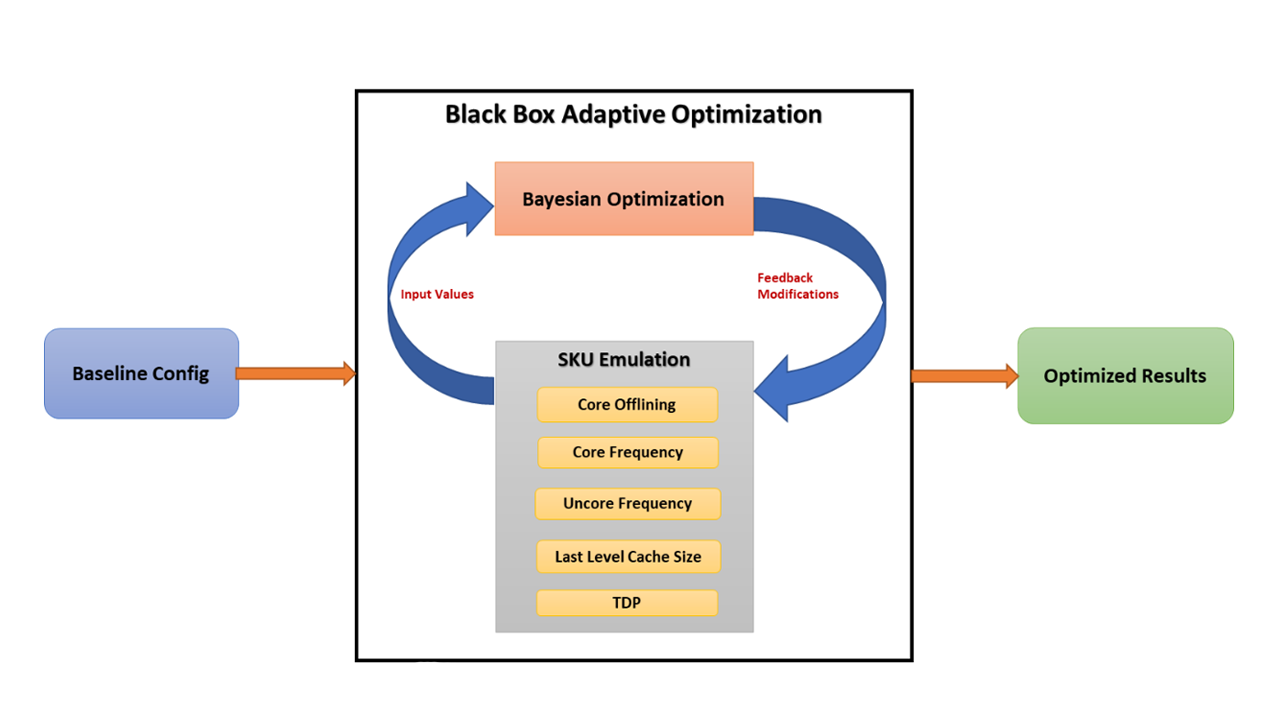
Figure 1. Overview of the Black Box Optimization process
Background
One of the customers was evaluating Intel® Xeon® Scalable Processors for maximum performance per Watt using a cloud benchmark. Traditional approach for this type of work is to run the workload on as many Intel Xeon Scalable Processors SKU’s as possible to find the optimal SKU. The entire process took over 10 weeks before landing on a SKU that fit the performance requirement and TCO model. The testing process was tedious, cumbersome and error prone since it involved several CPU swaps and changing the BIOS settings manually. The new proposed approach was implemented and tried with the same workload. After the new environment is setup, the whole optimization process was fully automated without any human intervention and the comparable results emerged in two days. Figure 2 shows the overall automated process flow.
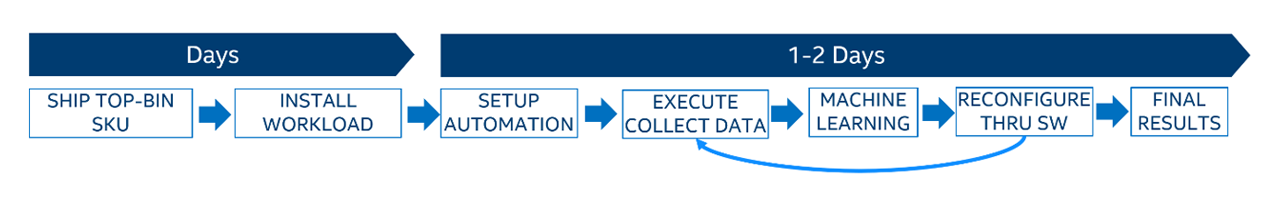
Figure 2. Overall Process Flow
SKU Emulation
Intel processors are generally manufactured in a wide variety of flavors to cater to wide market needs. Each flavor (SKU) comprises a judicious combination of capabilities such as core count, LLC, clock frequency, thermal design point (TDP), etc. engineered into a chip. SKUs represent a specialization or customization targeting a range of usages. For example, different SKUs may have a different number of processors. Sometimes SKUs may have custom requirements for motherboards, firmware, etc. Since Intel is in many different markets, it is not unusual to have a large number of SKUs – e.g., besides off-roadmap and custom-built SKUs, there are over 50 standard SKUs for Intel Xeon Scalable Processors. Producing many SKUs is itself complicated and costly, but it is not sufficient. Customers like to make decisions on SKUs for their infrastructure based on various parameters such as performance, power consumption, cost etc. Practically, they do so by sampling a bunch of the SKUs which they think may be beneficial, based on historical data, and perform rigorous testing with their representative set of workloads. We also then enable customers to meet function and cost design points using those SKUs by equipping them with a range of machines which they use for design validation, tuning, performance and power evaluations, and various other engineering activities. While all these steps are critical for achieving design wins, the entire enabling sequence is a very difficult and expensive process.
Typically, the major critical features that define a SKU include the followings:
- Number of cores
- Core frequency turbo ratios
- Last level cache size
- Un-core minimum and maximum frequency limits
- RAPL (Running average power limit)
Each of the above critical features have tunable values that are exposed through MSRs (model specific registers) and can be found in the Intel SDM (Software development manual)4. With the ability to control each of these features independently, we can understand the sensitivity of each to the workload’s tuning objective, be it performance or power. Modifying each feature can be done independently through MSRs mentioned below.
Number of Cores
The desired number of cores can be disabled in the OS by off-lining them at runtime. This can be only done in Linux* environment. Example: echo 0 > /sys/devices/system/cpuX/online where ‘X’ refers to the core number that user wants to offline. If Hyper-Threading is enabled, the corresponding logical processor on the system needs to be disabled as per the thread mapping defined on the given OS. This mapping can be determined on a Linux system using /sys/devices/system/cpu/cpuX/topology/thread_siblings. The offline process chosen here is top-down where the cores with higher core-id is disabled first along with its corresponding hyperthread if present till the required number of cores are achieved.
Core Frequency Turbo Ratios
The Core frequency (Turbo Core ratio) is defined with the help of 2 MSR registers: (0x1ADH and MSR 0x1AEH.) MSR 1ADH defines the frequency ratio limits and MSR 1AEH defines the active core ranges corresponding to those ratios.
In the adaptive optimization technique, we set the turbo core ratio fixed for all the cores. For example, the turbo core ratio for SKU 8180 that has 28 cores per package is 0x2021232323232426, which corresponds to turbo core ratio below:
Table 1. Turbo core frequency ratio for 8180 (default)
| 1AEH (No. of cores active) |
2 | 4 | 8 | 12 | 16 | 20 | 24 | 28 |
| 1ADH (GHz) (Value in hex) |
3.8 |
3.6 |
3.5 |
3.5 |
3.5 |
3.5 |
3.3 |
3.2 |
Now, if we want to set the core frequency to 2.9 GHz, we will set the MSR 1ADH to 0x1d1d1d1d1d1d1d1d. This ensures that the system will run at the fixed frequency of 2.9 GHz.
Table 2. Turbo core frequency ratio for 8180 after modifying core frequency
| 1AEH (No. of cores active) |
2 | 4 | 8 | 12 | 16 | 20 | 24 | 28 |
| 1ADH (GHz) (Value in hex) |
2.9 |
2.9 |
2.9 |
2.9 |
2.9 |
2.9 |
2.9 |
2.9 |
The above MSR manipulation works for non-turbo frequency ratios. Today, there are no MSRs to control AVX frequencies.
Last level cache size
Changing the last level cache size can be achieved by taking advantage of Cache Allocation Technology (CAT) in Intel Resource director technology. Please refer to Section 17.17 of Intel Software Developer Manual (Intel SDM)4 for more information regarding the CAT. The MSR C90H and C91H defines the class of service (COS) as shown below in Figure 3.
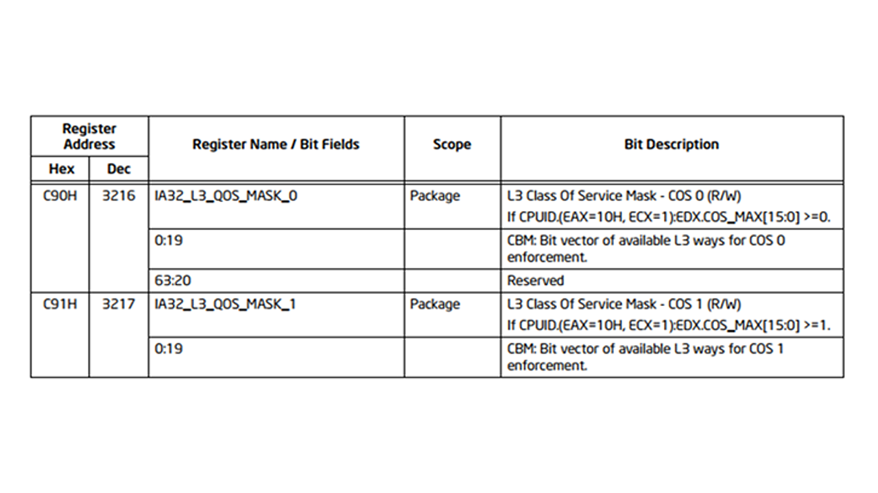
Figure 3. Cache QoS Class of Service (Intel SDM)
By default, all cores are present in class of service C90 (class 0). The cache can be reduced by cutting number of ways per cache set. For example, Intel Xeon Scalable Processors or second generation Intel Xeon Scalable Processors architecture defines 11 ways of cache, the default value of MSR C90H sets to 0x7ff. The MSR C90H may be changed to allocate the ways of cache to a given class of service. As per the table in Figure 4. The C90H MSR can be set to 0x7f8 to enable 8 ways i.e., 28MB of LLC cache. The cache may be sliced by ways which means that the MSR only accepts consecutive 1’s, corresponding to the ways in the cache. This limits the values that the cache can be sliced to as shown in the table in Table 3.
Table 3. Cache QoS table for Intel Xeon Scalable Processors 8180
| Cache QOS COS | Ways | Size in MB |
| 0x7ff | 11 | 38.5 |
| 0xfe | 10 | 35 |
| 0x7fc | 9 | 31.5 |
| 0x7f8 | 8 | 28 |
| 0x7f0 | 7 | 24.5 |
| 0x7e0 | 6 | 21 |
| 0x7c0 | 5 | 17.5 |
| 0x780 | 4 | 14 |
| 0x700 | 3 | 10.5 |
| 0x600 | 2 | 7 |
| 0x400 | 1 | 3.5 |
Uncore Frequency
The uncore frequency limits are defined by the MSR 0x620H. According to Intel SDM, this register defines max-ratio and min-ratio which represents the wildest possible range of uncore frequencies. Writing to the bits 0:6 for max-ratio and bits 8:14 for min-ratio (see Figure 4) allows the software to control the minimum and maximum frequency that the hardware will select.
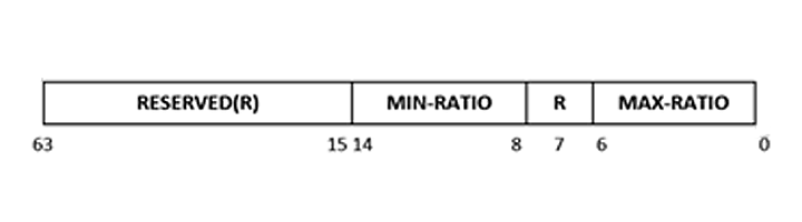
Figure 4. MSR descriptor for uncore frequency limits
These min and max ratios can be modified at runtime to reflect the desired processor values. This will make sure that the system doesn’t go beyond the defined max or min value of uncore frequencies. In the current settings the min and max values are set to the same values ensuring the system runs at the defined uncore frequencies.
RAPL (Running Average Power Limit)
This can be done by modifying the registers that define the running average power limit (RAPL) for the processor in terms of 2 power limits – PL1 for long duration and PL2 for very short durations. Uncore frequencies in modern processors like Intel Xeon Scalable Processors are controlled independently of the core frequency and limited by the TDP (Thermal Design Power) of the processor. Limiting the RAPL values maintains the same power limits during emulation of the desired SKU, thus maintain the correct core and uncore frequency governance.
- The MSR_PKG_POWER_LIMIT (section 14.9.3 Intel SDM) MSR 610H (as shown in Figure 4) allows the software to define the power limits for the package domain. The RAPL (running average power limit) for Power Limit 1 (PL1) can be modified by changing the bit 0-14 of the MSR 610H as per the TDP defined for target SKU. The 63rd bit (lock bit) of the MSR needs to be unset for allowing the software to enforce the power limit settings.
- For example, to set a TDP of 150W on a processor whose current TDP is 205W. The TDP change can be achieved by modifying the MSR 610H: 0x387b000148668 0x387b0001484B0 for the Power limit 1. The same methodology is applied for PL2 as well, which is usually 1.2x times PL1.
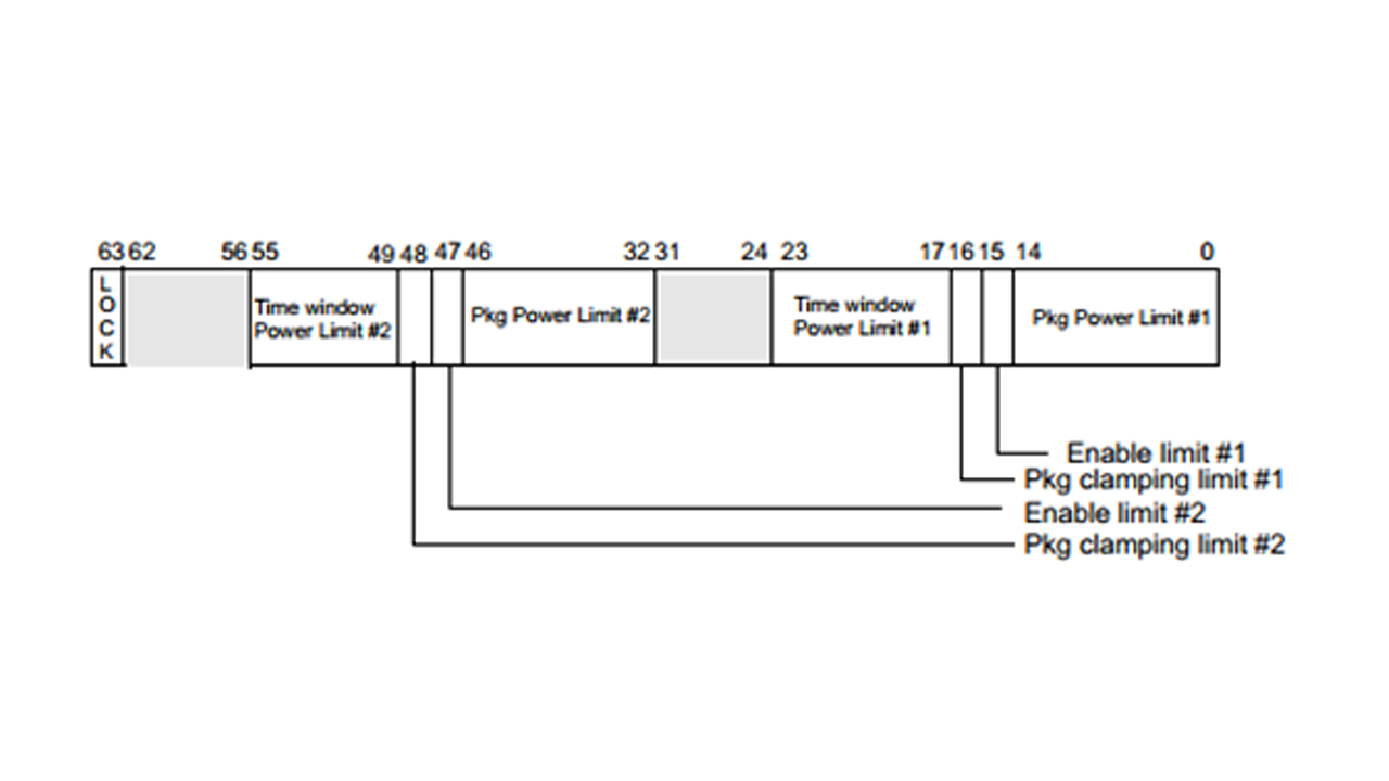
Figure 5. MSR descriptors for RAPL programming
Adaptive Optimization
Although SKU emulation significantly reduces the time and complexity of SKU selection, it does not address the time and expertise required to run through all possible combinations of configuration options. This section describes the basic method used to automatically configure the system for maximizing the given objectives by adjusting input parameters that can impact the performance.
Gaussian Process
Black box optimization refers to finding the optimal solution (max or min) to an objective function f(x) where any analytical expression for f nor its derivatives are known and the only way to get f(x) is restricted to sampling at a point x with noisy response. We could sample as many points if fis cheap to evaluate. Unfortunately, most benchmarks take considerable amount of time to evaluate and we need to minimize the number of sampling as much as possible in order to find a solution in a reasonable amount of time. There are many algorithms that are tried, but Bayesian optimization, one of the popular methods, is used in this paper. Bayesian optimization consists of calculating the mathematical model (surrogate model) estimating what the function looks like from the past samples, and a novel method to suggest next sampling point where an improvement over the current best observation is likely to happen. One of the popular surrogate models is Gaussian Processes which define a prior over functions representing our belief without any prior knowledge. There are a lot of math behind it 1, 2, 3 for further readings.) Figure 6 shows the case of multivariate gaussian distribution with mean vector (µ = 0) and sigma (σ = 1). 10 random functions are drawn from the distribution. What this figure means is that the average of all such (infinite number of) functions will be 0 and 95% of them all lie within the shaded region.
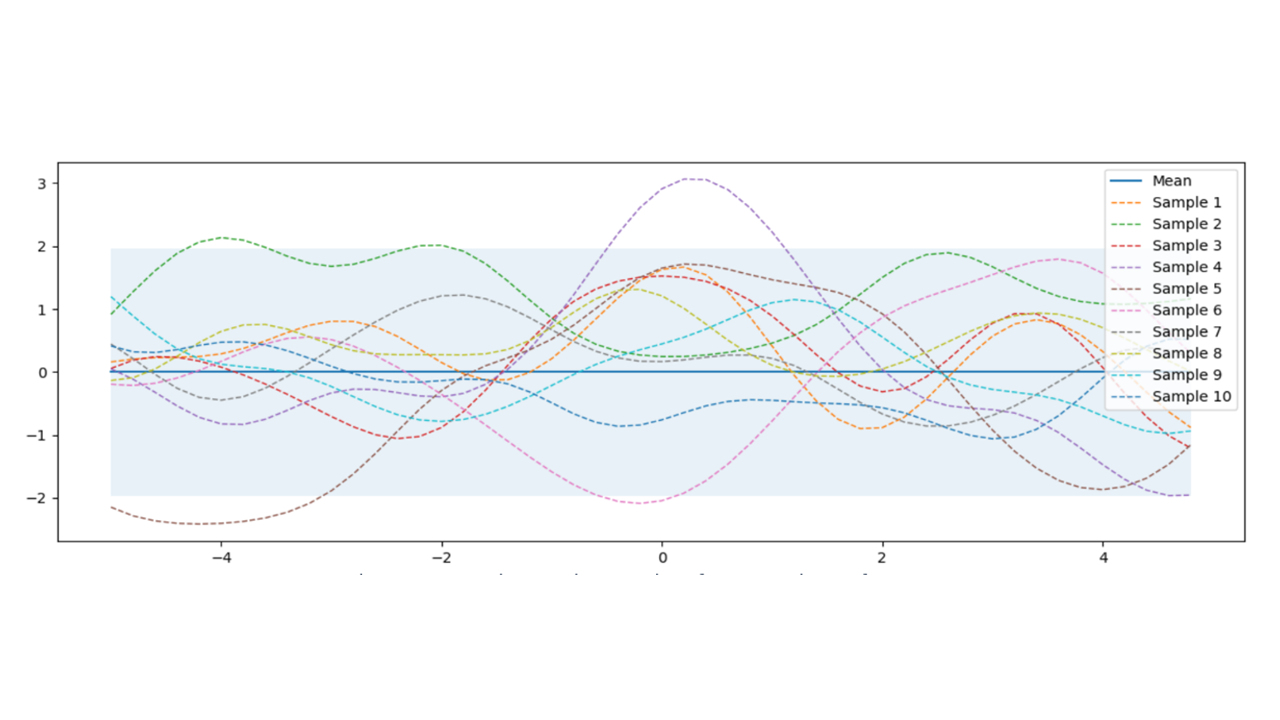
Figure 6. Gaussian Process priopr without training data and 10 random functions drawn from it
By itself, it’s not very useful, but this can be used with conditional probability (Bayesian rule) to calculate posterior to predict the probability of any unknown place given the sampled data as in Figure 7.
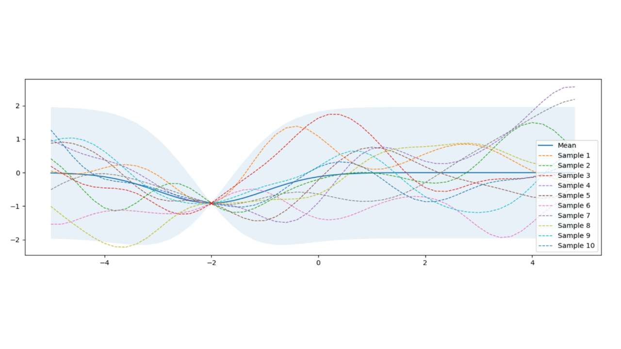
Figure 7. Gaussian Process posterior after 1 evaluation at -2
This provides a tool to predict not only the function’s shape µ (solid line), but also uncertainty σ (shaded area) that can be used to calculate where to evaluate in the next iteration. The whole idea around Bayesian optimization is that any two inputs close to each other has similar output, inevitably creating a curve. Furthermore, any points close to the actual samples have higher certainty than the points farther away, creating football-shaped regions around the evaluated places. Then, Bayesian optimization becomes the process of refining GP in an efficient way to find the optimum with as few evaluations as possible.
Acquisition Function
In order to determine where to sample next in the search space, an acquisition function is used. One extreme case of acquisition function is to directly use the predicted mean - calculate the maximum of the predicted mean, evaluate the function at that point, and feedback the results to the gaussian process in the next iteration. This will exploit the current maximum but end up with local maxima quickly. Another extreme will be to choose the point with maximum uncertainty. This is guaranteed to find the global maximum but will end up exploring the entire search space, beating the purpose of efficient optimization. One of the practical and easy to explain method is to calculate the maximum of the weighted sum of µ and σ.
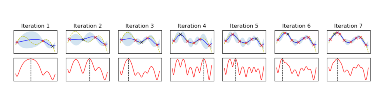
Figure 8. Bayesian optimization with UCB. The progress moves from left to right. Upper charts represent Gaussian process. Red dotted line is the real (imaginary) function. Red x are the training samples, while Black x is the last sample. Lower charts represent acquisition function (weighted sum of predicted mean and variance,) basically followng the Upper Confidence Bound (UCB). The argmax of the acquisition is used to sample in the next interation.
In figure 8, upper charts represent Gaussian process with samples. As the training data points are added, the model is getting refined. Note that it doesn’t get stuck to a local maximum and explores multiple peaks naturally, settling down to global maximum eventually. This example is searching for the maximum. If the minimum is sought after, you can follow the minimum of the lower bound and it’s called Lower Confidence Bound (LCB) method. This example just has one variable for the sake of description, but it can be expanded to multiple dimensions.
Given a number of well-defined parameters (X-axis) and performance metrics (Y-axis,) any optimization problem with multiple variables can be optimized with this method based on the assumption that similar settings produce similar outputs.
Performance measured as throughout is no longer the only requirement in practice in the industry. Most cloud workloads have stringent constraints on latency, throughput, power and may be other metrics in order to achieve higher TCO (Total Cost of Ownership). Typically, variety of CPUs are evaluated by running the customer workload or a proxy workload or a benchmark before selecting a SKU and optimizing for the desired metrices. This process is not only overly time consuming and expensive, sometimes CPU samples are not available during the early stage of manufacturing, which limits the ability to select the optimal CPU for the workload. And tuning the hardware for N parameters takes several iterations, seeks knowledge of hardware register programming, hardware resets, often making it hard to automate the process. Adaptive Optimization framework with SKU emulation can do the same by integrating the benchmark or a proxy workload with the workload constraints.
Next two sections illustrate the application of the machine learning (ML) in conjunction with SKU emulation to two of the real-world problems.
Case Study 1
We evaluated the framework on a customer proxy workload which was previously manually tuned for Performance per Watt. The workload performance is measured as RPS (Requests Per Second) for a certain type of web requests and goal is to achieve maximum RPS at the lowest power, while maintaining latency SLA (Service Level Agreement) and minimum throughput defined by the customer. In the absence of AO framework, we invested weeks in swapping CPUs, tuning power, frequency to select the right SKU to achieve optimal performance per Watt on the proxy workload. The end result was a custom Xeon SKU that fit the customer criteria the best, which included studying core-frequency scaling of the workload and testing against a handful of CPUs. Once we integrated the same workload into AO and defined the requirements, the framework was quickly able to derive the number of cores, core frequency, uncore frequency and power to maximize performance per Watt. This exercise took less than a day to come to the same conclusion that we had arrived at, without manual interventions. Another advantage of the method is that it can converge to a SKU setting that does not exist in the roadmap by learning sensitivity to core count, frequency and power, and can be used to defining a new custom CPUs.
Case Study 2
For this case study, we used adaptive optimization methodology on a customer workload that was latency sensitive in nature. As mentioned earlier there are five key components (number of cores, LLC (Last Level Cache) size, core frequency, un-core frequency and power) that can define a SKU. Our objective in this case study was to find the workload sensitivities to these five components and thereby aid the customer in SKU selection. The workload was a single node compute intensive steady state workload packaged in a Docker* container. It has a component that launches multiple server instances and the throughput is the server instances per core. We also ensure that while finding the maximum throughput on a given SKU, we also meet customer’s SLAs. We start with collecting a baseline on a given SKU matching the customer’s performance. We feed this baseline to the AO framework and manually define the acceptable ranges of the five key components we are interested to evaluate against. The ranges specified define the search space for the ML framework. The ML black-box algorithms run multiple iterations learning and making optimal decisions to maximize the throughput. Between each iteration we used the software-based capability to alter the five key components based on the optimal decisions made by the ML algorithms. Within a day of running multiple iterations, the AO framework converged and produced a 13 percent improvement over the customer’s baseline SKU. We also learnt the workload sensitivities, the results indicated that the workload benefitted from higher LLC size and higher frequencies. Within a day’s effort we were able to understand the workload sensitivities without having to perform tedious manual experiments on different SKUs for days together. One other advantage of this approach is that the ML framework takes care of learning and optimizing over different combinations of the five parameters (cores, LLC size, core frequency, un-core frequency and power). Manually running these experiments would make it tedious and time consuming to learn the effect of multiple parameters over wide ranges. We would have to manually swap parts and study one parameter at a time.
Conclusion
Intel SKUs are released in a generally optimized state and the actual performance or efficiency will depend on the nature of the SW that it’s running. Finding the right processor configuration and SKU has been always a time consuming and challenging work and an adaptive optimization approach based on Machine Learning was presented to automate the process. As of this writing, we are expanding the method to include other Hardware, BIOS, and Software components to provide an automated configuration of the system that’s customized for the specific needs at hand.
References
- Eric Brochu, Vlad M. Cora, Nando de Freitas, A Tutorial on Bayesian Optimization of Expensive Cost Functions.
- Jonas Mockus, Application of Bayesian approach to numerical methods of global and stochastic optimization.
- Donald R. JonesMatthias SchonlauWilliam J. Welch, Efficient Global Optimization of Expensive Black-Box Functions.
- Intel® 64 and IA-32 Architectures Software Developer Manuals.