
On October 24-25 in München, technical experts from around the world will gather at the Design and Verification Conference and Exhibition ( DVCon Europe) to share the latest developments in electronic design automation (EDA) languages, methodologies and tools. The program covers a lot of different topics, and two of my colleagues and I look forward to presenting the following papers:
- I will address temporal decoupling in virtual platforms in the Virtual Prototyping session
- Evgeny Yulyugin will present his work on optimizing direct execution-based virtual platform instruction-set simulation in the presence of complicated instructions
- Roman Popov will talk about hardware construction (algorithmic circuit generation) in synthesizable SystemC
I expect a great conference this year, just like previous years! I will be talking about temporal decoupling in virtual platforms, which is something I have wanted to do for years. For some reason, until now I have never quite got around to writing down what we have learnt about the topic of the years.
What is Temporal Decoupling?
Temporal decoupling is a key technology in virtual platforms. It has been used since at least the late 1960s to speed up the simulation of a system featuring multiple processor cores or multiple parallel processing units.
Temporal decoupling is an optimization that increases the performance of the virtual platform, but it also affects the precise semantics of the simulation. In the talk and paper, I discuss what temporal decoupling is, and how the use of temporal decoupling affects the behavior of the platform—and in particular, the software running on the virtual platform.
The Need for Performance
In a virtual platform, we simulate the hardware of a computer system so that we can run the software without the real hardware. In general, we can have multiple boards and networks inside the virtual platform system:
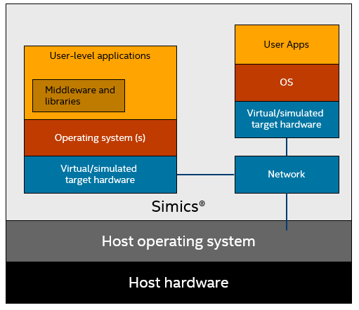 A virtual platform system can simulate multiple boards and networks. |
Target hardware and workloads for virtual platforms are often rather large; examples include running a thousand target machines in a single simulation, or big database benchmarks and distributed business systems. Thus, performance is crucial to getting value out of virtual platforms.
Digging into Temporal Decoupling
With temporal decoupling, a system with multiple target processors (or other active units like accelerators) is simulated on a single host processor. Temporal decoupling lets each target processor run multiple simulation steps or cycles before handing over to the next processor. The image below illustrates the idea, using five processors spread across three boards.
|
|
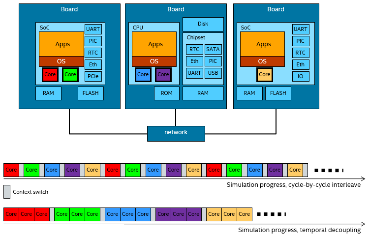
In a naïve execution model, the simulator would run each processor for one cycle and then switch to the next. This would closely approximate the parallel behavior seen in the real world, but at a very high cost. Each context switch between processors would involve the simulator kernel, leading to a very high overhead-to-useful-work ratio. Second, by only running a single cycle at a time, each processor would get very poor locality, and it would be meaningless to try to speed-up the execution with faster techniques like just-in-time (JIT) compilation because each unit of translation would be a single instruction.
Performance Benefits
Keeping everything else constant, increasing the time quanta can radically increase performance. The chart below (in log-log scale) shows the relative speed as the time quantum goes from one cycle to two million cycles. The target system is a four-core Intel® Core® processor-based PC running Linux* and running a threaded program that keeps all cores busy at close to max-content.
|
|
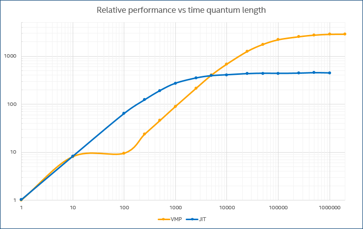
The curve labelled “JIT” indicates the speedup achieved using just-in-time compilation, and the curve labelled “VMP” indicates the speedup for Wind River Simics® VMP technology. VMP uses Intel® Virtualization Technology for Intel® 64 and IA-32 architectures (Intel® VT-x) to execute instructions directly on the host. For JIT, the speedup plateaus out at about 400x, and for VMP at around 2800x.
Even a speedup of 100x is a big deal: it means the difference between a run that takes 1 minute and a run that takes more than an hour and half. It is the difference between “interactive” and “batch” modes.
Changed Semantics?
The general effect of temporal decoupling is to add a latency when an event or a state change from one processor becomes visible on another processor. For example, if software on one processor writes a value to memory, software on another processor will not see it until it gets to run its time quantum. This effect means that software might see time differences between processors that are bigger than they would be on real hardware.
In principle, this sounds bad, and quite a few papers on discrete event simulation have strived to define ways in which errors can be kept under control, detected, and even backtracked to correctness. In practice, temporal decoupling has worked very well in virtual platforms, for most workloads, for a very long time (as noted above, the first documented use is in the late 1960s).
However, most is not all. I remember my first time seeing a significant effect from temporal decoupling back in the mid-2000s, in the early days of multicore computing. We were experimenting with booting Linux on a simulated dual-core target and optimizing the performance using longer time quanta. Initially, as the time quantum length was increased, the boot time decreased. That was expected because the simulator ran faster. But from 100k cycle time quanta, the boot time as observed on the host started to increase, as shown by the yellow line in the graph below:
 In this early-days example, the boot time as observed on the host and the number of target instructions executed started to increase beyond a 100k cycle time quantum. |
The reason for this loss of performance at longer time slices is shown by the blue line. When the time quantum was set to 100k cycles or more, the target system started to execute many more instructions during the boot. From a performance perspective, the benefit of a longer time quantum was negated by executing additional instructions. From a functionality perspective, the system was sufficiently affected by long time quanta that it made no sense to use a time quantum larger than 10k.
The culprit was a piece of code in the Linux kernel that tried to calibrate the time difference between cores: when the time quantum got large, this code started to see large time differences between cores which in turn made it loop many times to find a stable time difference. Eventually, it did get through for all cases, but it took more and more target time, as the time quantum increased. It was interesting to see this effect, and similar things do come up from time to time. Note that this particular algorithm was removed from later versions of the Linux kernel.
Learn More at DVCon Europe
At DVCon Europe, I will go into more depth about how temporal decoupling works, and I will cover some more examples of how temporal decoupling impacts target system semantics. I will share several techniques that have been developed to mitigate the effects of temporal decoupling on software that get employed in virtual platforms. I hope to see you at the conference!