Introduction
Caffe* is a deep learning framework developed by the Berkeley Vision and Learning Center. It is written in C++, and has a C++ API, as well as Python and MATLAB bindings.
The sources, samples, and documentation are available at the GitHub site https://github.com/BVLC/caffe. However, the samples alone and the documentation leave problems for new developers, along with a steep learning curve for developers to work through in order to use the framework for customized uses.
This document sets out to demonstrate, in two samples, how to configure Caffe and how to perform two custom training and classification tasks:
- Train a network with randomly generated XOR data and classify with the trained model
- Train a network with randomly generated shapes (squares and circles) data and classify with the trained model
This document does not set out to detail the architecture or primary usage (image recognition) of Caffe, as that information is abundantly documented at http://caffe.berkeleyvision.org.
The accompanying source codes assume that the reader is familiar with the Caffe C++ API, Google* Protocol Buffers (protobufs), and the building, running, and installation of Caffe in an Ubuntu* 16.04 LTS environment. In addition, it is assumed that the reader is familiar with the CMake facility, as it forms the backbone of how the samples are built. Finally, OpenCV v3.0 is required to be installed on the system, as the shapes require it for build and execution.
Overview
There are four steps in training a network using Caffe:
Step 1 - Data preparation: In this step, data is prepared and stored in a format that can be used by Caffe. We will write a C++ app that will handle both data pre-processing and storage.
Step 2 - Model definition: In this step, we compose a network topology/architecture and we define its parameters in a configuration file with the extension .prototxt.
Step 3 - Solver definition: The solver is responsible for model optimization. We define the solver parameters in a configuration file with the extension .prototxt.
Step 4 - Model training: We train the model by executing one Caffe command from the terminal. After training the model, we will get the trained model in a file with the extension .caffemodel.
After the training phase, we will use the .caffemodel trained model to make predictions of new, unseen data. We will write a C++ app to perform this.
For the purposes of the samples, several of these steps are encapsulated inside shell scripts to assist the reader in the execution of the custom programs they call upon.
Review of Sample Source Tree
The top level (root) of the sample tree is caffe-cpp-samples. Immediately beneath that is the /src directory. Inside the /src directory there are the directory names xor and shapes which, respectively, hold the code and scripts for the samples.
The CMake file, called CMakeLists.txt, contains a minimal set of instructions to build the samples and call upon the find_package() functionality to look for OpenCV and Caffe directories and definitions.
Building the samples is done by executing the following on the command line at project root:
cmake .
make all
XOR Sample
The purpose of the XOR sample is to demonstrate a simple network topology that contains hidden networks and performs the non-trivial evaluation of the XOR logical function. For an historical and mathematical motivation for this sample please refer to Appendix 1: Perceptrons and XOR Logic.
The XOR sample is organized into three steps:
- Generate training data
- Train the network
- Classify using the network
Generate training data
./generate.sh
This script calls on the executable built from generate-random-xor-training-data.cpp, generates 1000 random XOR samples, and puts the resulting data into two LMDB databases, xor_lmdb_train and xor_lmdb_test, divided into 500 samples each.
Possible values for the samples for the XOR function are from the following truth table:
|
In1 |
In2 |
Out |
|---|---|---|
| 0 | 0 | 0 |
| 0 | 1 | 1 |
| 1 | 0 | 1 |
| 1 | 1 | 0 |
where Out is the same as the label.
Train the network
./train.sh
This default training calls upon the already built caffe train, and the script uses the settings from the solver.prototxt to train the network defined by train-test.prototxt. In the end it should give an accuracy of 1 and the loss should minimize to a really low number approaching 0.0.
Classify Using the Network
./classify.sh
This default classification script calls on the executable built from classify-xor.cpp, classifies all four possible Input combinations (see table above) using the trained model and the network from deploy.prototxt, and shows the values and whether it was classified correctly.
Shape Example
The shape example is similar in organization to the XOR sample, that is, it is broken down into three steps:
- Generate training data
- Train the networks
- Classify some data with the trained model
Generate training data
./generate.sh
This default generate script calls on the executable built from generate-random-shape-training-data.cpp, generates 1000+ random samples, and puts them into two LMDB databases, shape_lmdb_train and shape_lmdb_test, equally divided. The samples are a square kernel of all shapes and the background around the shapes. Each shape is labeled, 1 for squares, 2 for circles and 0 for background.
Train the network
./train.sh
As in the XOR sample, this default script calls on caffe train and uses the settings from the solver.prototxt to train the network defined by train-test.prototxt. In the end it should give an accuracy of 1 and the loss should minimize 0.0.
Classify some data with the trained model
./classify.sh
This classification script encapsulates the built executable from classify-shape.cpp and classifies a random generated image with squares and circles, using the trained model and the network from deploy.prototxt. In the end it shows the classification result image and the classification error percentage.
Conclusion
Caffe is a deep learning framework made with expression, speed, and modularity in mind. However, these features come at the expense of presenting a developer with a steep learning curve. This document presents to the reader enough working knowledge to build and run two samples where each require the use of a custom network topology.
The reader is encouraged to read through the copious comments in the provided source codes and prototxt files for details of how to specifically code for the Caffe C++ API and set up the custom network topologies.
Appendix 1: Perceptrons and XOR logic
The advent of multilayer neural networks sprang from the need to implement the XOR logic gate. Early perceptron researchers ran into a problem with XOR, the same problem as with electronic XOR circuits: multiple components were needed to achieve the XOR logic. With electronics, two NOT gates, two AND gates, and an OR gate are usually used. With neural networks, it seemed that multiple perceptrons were needed (in a manner of speaking). To be more precise, abstract perceptron activities needed to be linked together in specific sequences and altered to function as a single unit. Thus were born multilayer networks.
Why go to all the trouble to make the XOR network? Two reasons: (1) a lot of problems in circuit design were solved with the advent of the XOR gate, and (2) the XOR network opened the door to far more interesting neural network and machine learning designs.
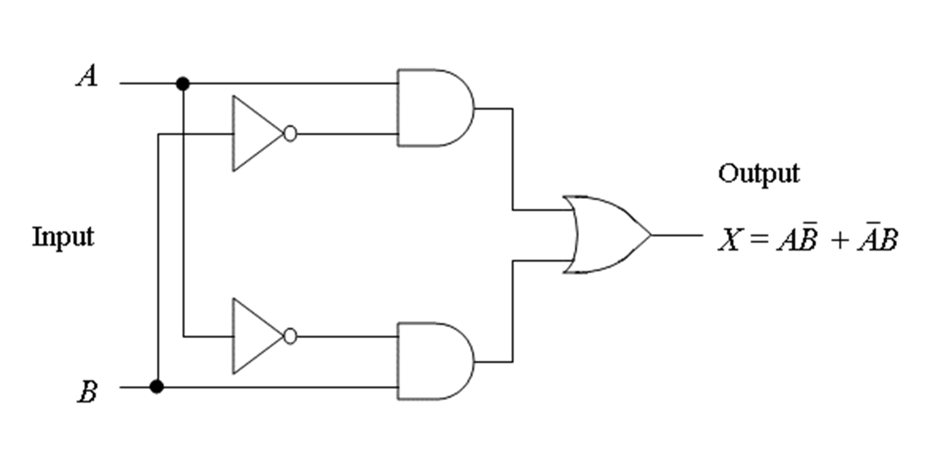
Figure 1: XOR logic circuit (Floyd, p. 241).
If you're familiar with logic symbols, you can compare Figure 1 to Figure 2, and see how the two function alike. The two inverters (NOT gates) do exactly what the -2 is doing in Figure 2. The OR gate is doing exactly the same function as the 0.5 activation in the output unit of Figure 1. And everywhere you see a +1 in Figure 2, those together perform the same as the two AND gates in Figure 1.
While perceptrons are limited to variations of Boolean algebra functions including NOT, AND, and OR, the XOR function is a hybrid involving multiple units (Floyd, p. 241).
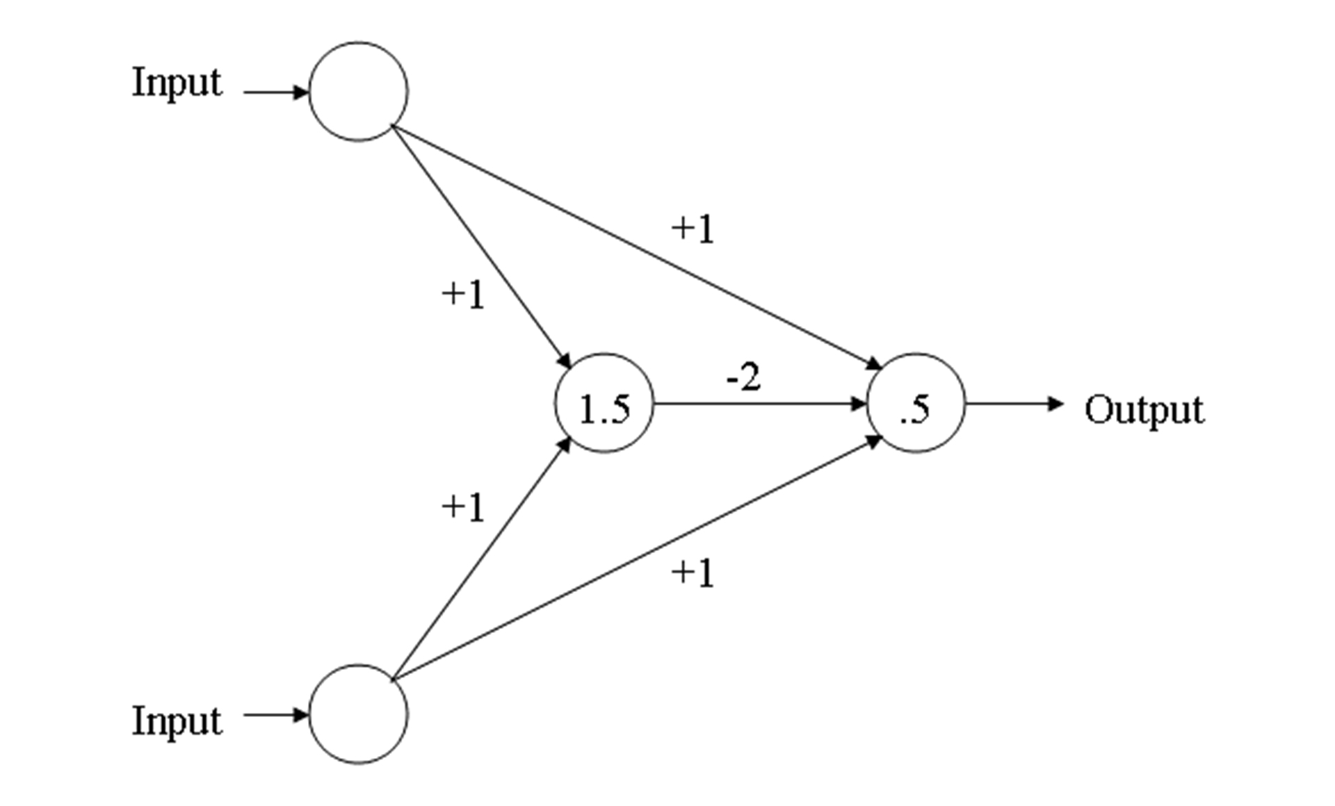
Figure 2: XOR Gate.
Note the center-most unit is hidden from the outside influence, and only connects via input or output units. The value of 1.5 for the threshold for the hidden unit ensures that it will be turned on only when both input units are on. The value of 0.5 for the output unit ensures that it will turn on only when a net positive input is greater than 0.5. The weight of -2 from the hidden unit to the output unit ensures that the output unit will come on when both inputs are on.
A multilayer perceptron (MLP) is a type of neural network referred to as a supervised network because it requires a desired output in order to learn. The goal of this type of network is to create a model that correctly maps the input to the output using pre-chosen data so that the model can then be used to produce the output when the desired output is unknown.
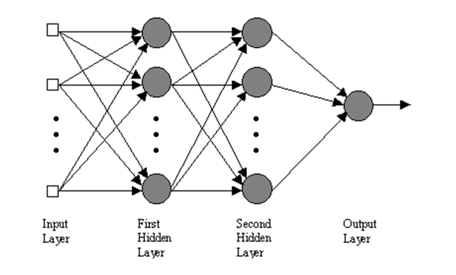
Figure 3: An MLP with two hidden layers.
As input patterns are fed into the input layer, they get multiplied by interconnection weights while passing from the input layer to the first hidden layer. Within the first hidden layer they get summed, and then processed by a nonlinear activation function. Each time data is processed by a layer it gets multiplied by interconnection weights, then summed and processed by the next layer. Finally the data is processed one last time within the output layer to produce the neural network output.
The MLP learns using an algorithm called backpropagation. With backpropagation, the input data is repeatedly presented to the neural network in a process known as training. With each presentation the output of the neural network is compared to the desired output and an error is computed. This error is then fed back (backpropagated) to the neural network, and used to adjust the weights in such a way that the error decreases with each iteration and the neural model gets closer and closer to producing the desired output.
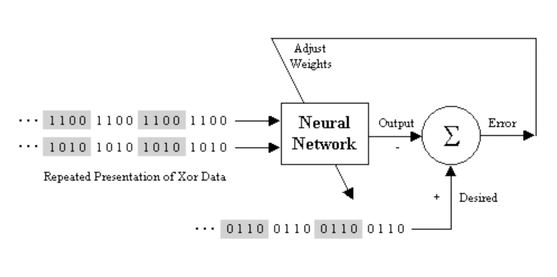
Figure 4: A neural network learning to model exclusive-or (XOR) data.
The XOR data is repeatedly presented to the neural network. With each presentation, the error between the network output and the desired output is computed and fed back to the neural network. The neural network uses this error to adjust its weights in such a way that the error will be decreased. This sequence of events is usually repeated until an acceptable error has been reached or until the network no longer appears to be learning.
Works Cited
Floyd, Thomas L. (2003). Digital fundamentals (8th ed.). New Jersey: Prentice Hall.
Rumelhart, D. E., Hinton, G. E. and Williams, R. J. 1986. Learning internal representations by error propagation. In Rumelhart, D. E., McClelland, J. L. (Eds.), Parallel distributed processing: Explorations in the microstructure of cognition. Vol. 1. Cambridge: MIT Press.