Overview
This is a tutorial to help developers improve the performance of their games in Unreal Engine 4 (UE4). In this tutorial, we go over a collection of tools to use within and outside of the engine, as well some best practices for the editor, and scripting to help increase the frame rate and stability of a project.
The goal of this tutorial is to identify where performance issues occur and provide several methods to tackle them.
Version 4.14 was used in the making of this guide.
Units
For measuring improvements made with optimizations, frames per second (fps) and duration in milliseconds per frame (ms) are considered.
This chart illustrates the mapping between average fps and ms.
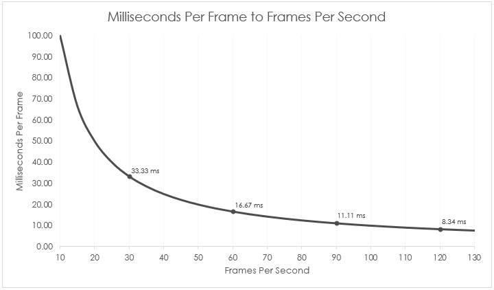
To find the ms of any fps, simply get the reciprocal of that fps and multiply by 1000.
![]()
Using milliseconds to describe improvements in performance helps better quantify level of optimization needed to hit the fps target.
For instance, with an improvement of 20 fps to a scene:
- 100 fps to 120 fps is an improvement of 1.66 ms
- 10 fps to 30 fps is an improvement of 66.67 ms
Tools
To get started, let’s look at three tools for understanding what is happening under the hood of the engine: UE4 CPU Profiler, UE4 GPU Visualizer, and the Intel® Graphics Performance Analyzers (Intel® GPA).
Profiler
The UE4 CPU Profiler tool is an in-engine monitor that allows you to see the performance of the game, either live or from a captured section.
Find the Profiler under Window > Developer Tools > Session Frontend.
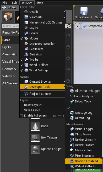
Figure 1: Finding the Session Frontend window.
In Session Frontend, select the Profiler tab.
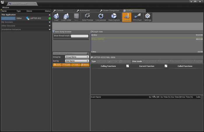
Figure 2: The Profiler in the Unreal Engine.
Now that we are in the Profiler window, select Play-In-Editor (PIE), then select Data Preview and Live Preview to see the data being collected from the game. Select the Data Capture option to begin capturing data from the game, and then deselect it to save that data for later viewing.
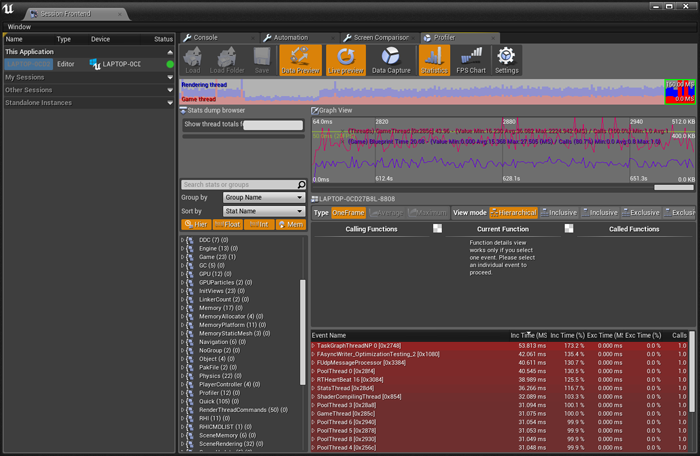
Figure 3: Viewing processes within the Profiler.
From the Profiler, the time of every action and call is reflected in ms. Each area can be examined to see how it affects the frame rate within the project.
For an in-depth explanation of the Profiler, see the Epic documentation.
GPU Visualizer
The UE4 GPU Visualizer identifies the cost of rendering passes and provides a high-level view of what is happening within a scene snapshot.
The GPU Visualizer can be accessed from the in-game developer console by entering ProfileGPU.

Figure 4: ProfileGPU console command.
Once the command is entered, the GPU Visualizer window pops open. It shows the time of each rendering pass within the snapshot and a rough idea of where in the scene those passes took place.
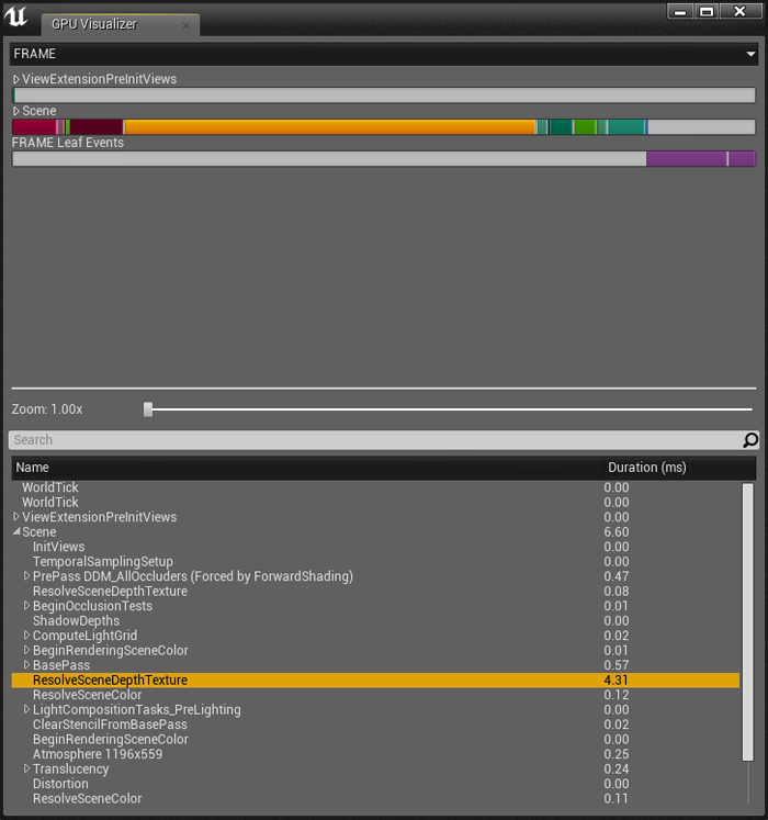
Figure 5: Viewing processes within the GPU Visualization.
As with the Profiler, identifying the items that take the most processing time will give clues about where to start optimization efforts.
For an in-depth explanation of the GPU Visualizer, see the Epic documentation.
Intel® Graphics Performance Analyzers (Intel® GPA)
Intel GPA is a suite of graphics analysis and optimization tools that help developers get more performance out of their graphics applications.
For this guide, we will focus on two aspects of the suite: the real-time Analyze Application and Frame Analyzer. To get started, download GPA from the Intel® Developer Zone. Once installed, build the Unreal project with the Development Build Configuration selected.
With the build complete, go into Analyze Application of the Graphics Monitor and select the executable location in the command line and run it.
The game will open normally, but now a statistics guide is visible in the top-left corner of the screen. To expand the display, press CTRL+F1 once for real-time metrics information, and again to get a list of keyboard shortcuts of experiments available to be applied as the game is running.
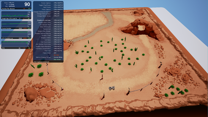
Figure 6: The Intel GPA overlay in game.
To get a frame to analyze in Frame Analyzer, two additional steps are needed in-game.
First is to turn on Toggle Draw Events. To do this, type ToggleDrawEvents into the game console.

Figure 7: ToggleDrawEvents console command.
Turning this on attaches names to the draw calls being made by the engine so that we have context when looking at the capture later in Frame Analyzer.
Finally, we capture a frame with the keyboard shortcut CTRL+SHIFT+C.
With the frame saved, open Frame Analyzer from the Graphics Monitor and select the frame to be loaded. After the capture is processed all the information about what occurred graphically within the frame presented.
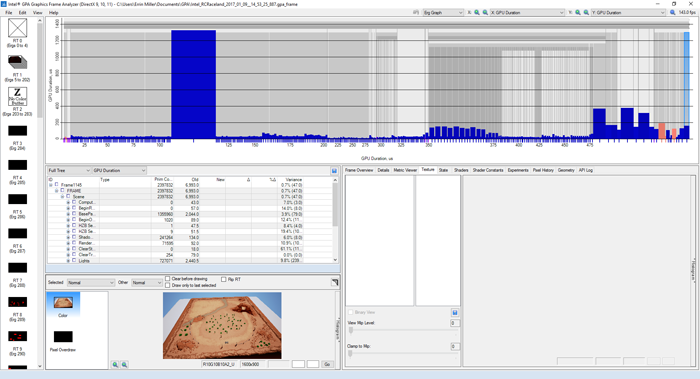
Figure 8: The Intel GPA.
For an in-depth explanation, see the Intel GPA documentation.
Intel GPA Usage Example
While it may look complicated seeing all the data in Intel GPA, we start by just looking at the bigger chunks of information first. In the top-right corner of the window, set the graph to be GPU Duration on the X and Y axes; this gives us a graph of which draw calls take up the most time in our frame.
In this example, a capture of a desert landscape scene, we see there is a massive draw call in the base pass. When the large draw call is selected, and Highlighted is selected in the Render Target Preview area, we see that the spike was caused by the landscape (highlighted in pink) within the scene. If we dive into the Process Tree List (just above the preview area) to find the selected draw call, we see that the landscape has 520,200 primitives and takes a GPU duration of 1,318.5 (1.3185 ms).
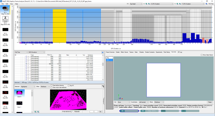
Figure 9: Finding the largest duration within the scene.
Once we identify what caused the spike we can try to optimize it.
As a first measure, the landscape is resampled down by using Manage Mode for the landscaping tool, which reduces its primitive count to 129,032. This reduces the GPU duration to 860.5, and gives an improvement of 5 percent to the scene.
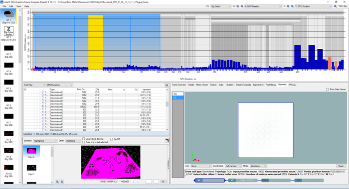
Figure 10: Seeing the decreased duration.
To continue to lower the cost of the landscape, we can also look its materials. The landscape has a layer blend material that uses thirteen 4096 x 4096 (4k) textures, which totals 212.5 MB of texture streaming.
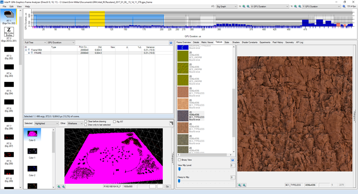
Figure 11: Viewing rendered textures in the Intel GPA.
By compressing all the landscape textures to 2048 x 2048 (2k), we reduced the GPU duration to 801.0 and got another improvement of 6 percent.
Reducing the texture streaming of the landscape to 53.1 MB and cutting the overall triangle count of the scene allowed the project to run better on Intel graphics. This is all while only decreasing the visual fidelity of the landscape by a small amount for the project.
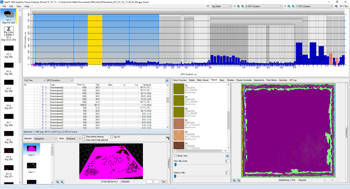
Figure 12: Seeing the decrease in duration with texture reduction.
Overall, just changing the landscape of the scene with the resampling and changes in textures, we got an optimization of:
- 40 percent (1318.5 to 801) reduction in the GPU duration of the landscape process
- An improved fps of 18 (143 to 161)
- A reduction of 0.70 ms per frame
Editor Optimizations
This part of the tutorial is to help developers improve the performance of their games in Unreal Engine 4 (UE4). We go over a collection of tools to use within and outside of the engine and some best practices for the editor to help increase the frame rate and stability of a project.
Forward Compared to Deferred Rendered
Deferred is the standard rendering method used by UE4. While it typically looks the best, there are important performance implications to understand, especially for VR games and lower-end hardware. Switching to Forward Rendering may be beneficial in these cases.
For more details on the effect of using Forward Rendering, see the Epic documentation.
If we look at the Reflection scene from the Epic Games* Marketplace, we can see some of the visual differences between Deferred and Forward Rendering.
Figure 13: Reflection scene with Deferred Rendering
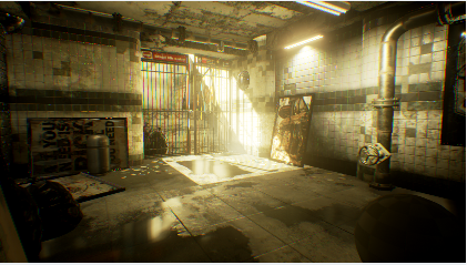
Figure 14: Reflection scene with Forward Rendering
While Forward Rendering comes with a loss of visual fidelity from reflections, lighting, and shadows, the remainder of the scene remains visually unchanged and performance increases may be worth the trade-off.
If we look at a frame capture of the scene using the Deferred Rendering in the Intel GPA Frame Analyzer tool, we see that the scene is running at 103.6 ms (9 fps) with a large duration of time being taken by lighting and reflections.
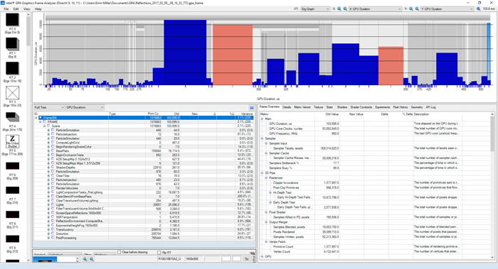
Figure 15: Capture of the Reflection scene using Deferred Rendering on Intel® HD Graphics 530
When we look at the Forward Rendering capture, we see that the scene’s runtime has improved from 103.6 to 44.0 ms, or 259 percent improvement, with most time taken up by the base pass and post processing, both of which can be optimized further.
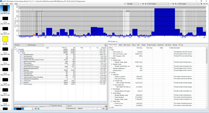
Figure 16: Capture of the Reflection scene using Forward Rendering on Intel HD Graphics 530
Level of Detail (LOD)
Static meshes within UE4 can have thousands, even hundreds of thousands, of triangles in their mesh to show all the smallest details a 3D artist could want to put into their work. However, when a player is far away from that model, they won’t see any of that detail, even though the engine is still rendering all those triangles. To solve this problem and optimize our game, we can use level of detail (LOD) to have that detail up close, while also showing a less intensive model at a distance.
LOD Generation
In a standard pipeline, LODs are created by the 3D modeler during the creation of that model. While this method allows for the most control over the final appearance, UE4 now includes a great tool for generating LODs.
Auto LOD Generation
To autogenerate static mesh LODs, go into that model’s details tab. On the LOD Settings panel, select the Number of LODs you would like to have.
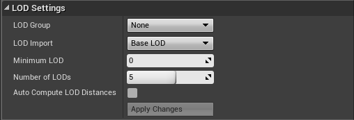
Figure 17: Creating autogenerated level of details.
Clicking Apply Changes signals the engine to generate the LODs and number them, with LOD0 as the original model. In the example below, we see that the LOD generation of 5 takes our static mesh from 568 triangles to 28—a huge optimization for the GPU.
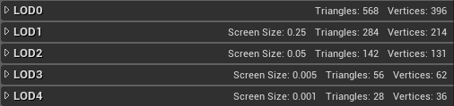
Figure 18: Triangle and vertex count, and the screen size setting for each level of detail.
When we place our LOD mesh in the scene, we can see the mesh change the further away it is from the camera.
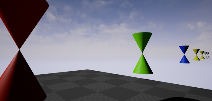
Figure 19: Visual demonstration of level of detail based on screen size.
LOD Materials
Another feature of LODs is that each one can have its own material, allowing us to further reduce the cost of our static mesh.
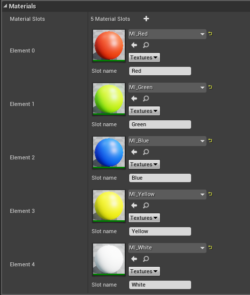
Figure 20: Material instances applied to each level of detail.
For example, the use of normal maps has become standard in the industry. However, in VR there is a problem; normal maps aren’t ideal up close as the player can see that it’s just a flat surface.
A way to solve this issue is with LODs. By having the LOD0 static mesh detailed to the point where bolts and screws are modeled on, the player gets a more immersive experience when examining it up close. Because all the details are modeled on, the cost of applying a normal map can be avoided on this level. When the player is further away from the mesh and it switches LODs, a normal map can then be swapped in while also reducing the detail on the model. As the player gets even further away and the mesh gets smaller, the normal map can again be removed, as it becomes too small to see.
Instanced Static Meshes
Every time anything is brought into the scene, it corresponds to an additional draw call to the graphics hardware. When this is a static mesh in a level, it applies to every copy of that mesh. One way to optimize this, if the same static mesh is repeated several times in a level, is to instance the static meshes to reduce the amount of draw calls made.
For example, here we have two spheres of 200 octahedron meshes; one set in green and the other in blue.
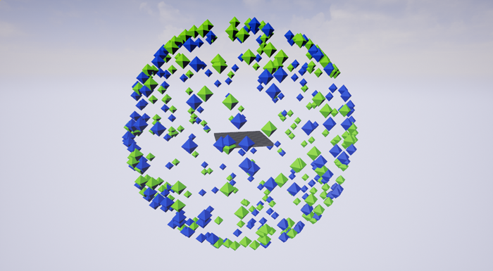
Figure 21: Sphere of static and instanced static meshes.
The green set of meshes is all standard static meshes, meaning that each has its own collection of draw calls.
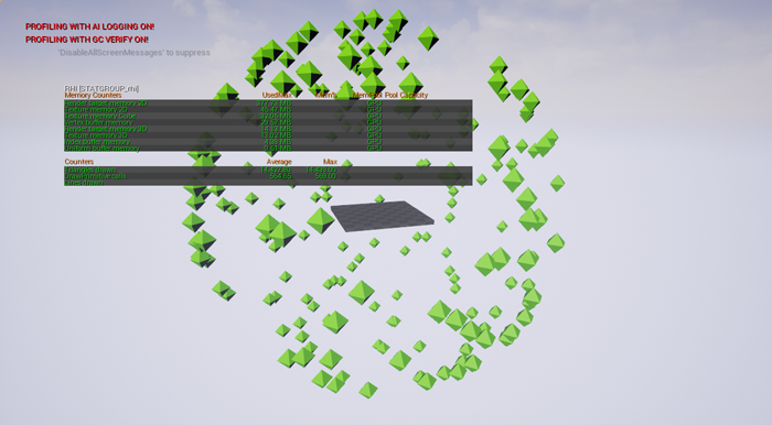
Figure 22: Draw calls from 200 static mesh spheres in scene (Max 569).
The blue set of meshes is a single-instanced static mesh, meaning that they share a single collection of draw calls.
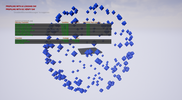
Figure 23: Draw calls from 200 instanced static mesh spheres in scene (Max 143).
Looking at the GPU Visualizer for both, the Base Pass duration for the green (static) sphere is 4.30 ms and the blue (instanced) sphere renders in 3.11 ms; a duration optimization of about 27 percent in this scene.
One thing to know about instanced static meshes is that if any part of the mesh is rendered, the whole of the collection is rendered. This wastes potential throughput if any part is drawn off camera. It’s recommended to keep a single set of instanced meshes in a smaller area; for example, a pile of stone or trash bags, a stack of boxes, and distant modular buildings.
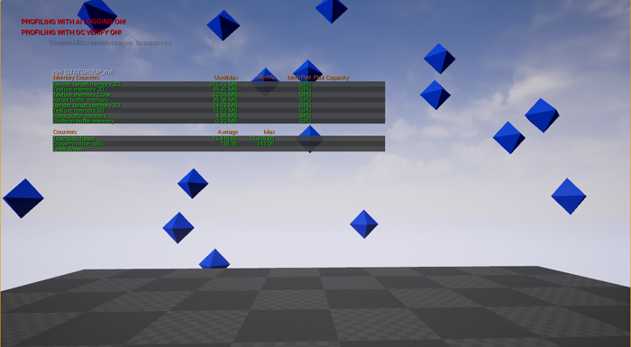
Figure 24: Instanced mesh sphere still rendering when mostly out of sight.
Hierarchical Instanced Static Meshes
If collections of static meshes that have LODs are used, consider a hierarchical instanced static mesh.
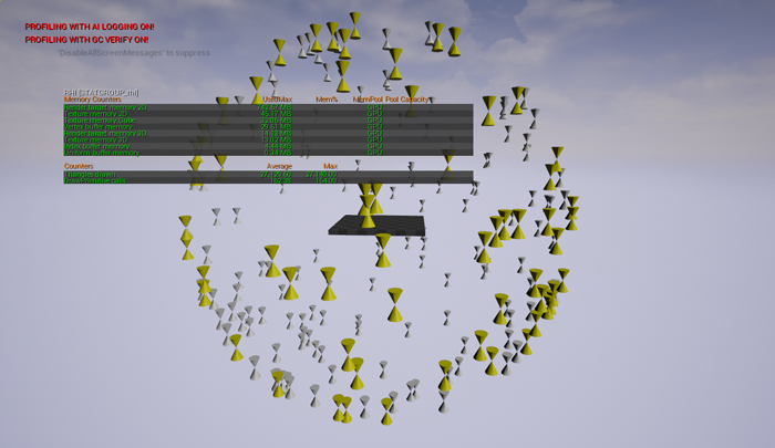
Figure 25: Sphere of hierarchical instanced meshes with level of detail.
Like a standard instanced mesh, hierarchical instances reduce the number of draw calls made by the meshes, but the hierarchical instance also uses the LOD information of its meshes.
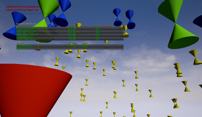
Figure 26: Up close to that sphere of hierarchical instanced meshes with level of detail.
Occlusion
In UE4, occlusion culling is a system where objects not visible to the player are not rendered. This helps to reduce the performance requirements of a game as you don’t have to draw every object in every level for every frame.
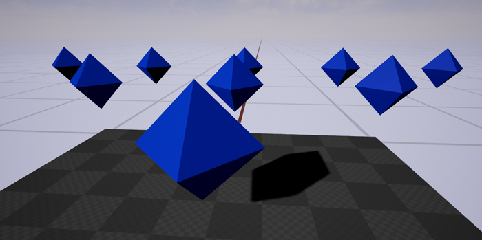
Figure 27: Spread of octohedrons.
To see the occluded objects with their green bounding boxes, you can enter r.VisualizeOccludedPrimitives 1 (0 to turn off) into the console command of the editor.
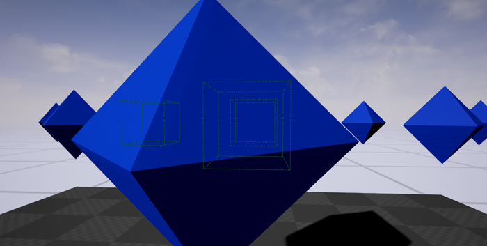
Figure 28: Viewing the bounds of occluded meshes with r.VisualizeOccludedPrimitives 1
The controlling factor of whether or not a mesh is drawn is relative to its bounding box. Because of this, some drawn objects that may not be visible to the player, but the bounding box is visible to the camera.
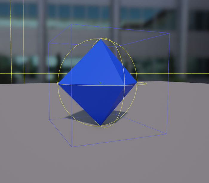
Figure 29: Viewing bounds in the meshes details window.
If a mesh needs to be rendered before a player sees it, for additional streaming time or to let an idle animation render before being seen, for example, the size of the bounding boxes can be increased under the Static Mesh Settings > Positive Bounds Extension and Negative Bounds Extension in the Mesh Settings window.
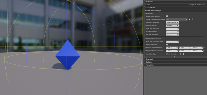
Figure 30: Setting the scale of the mesh’s bounds.
As the bounding box of complex meshes and shapes always extend to the edges of those meshes, creating white space causes the mesh to be rendered more often. It is important to think about how mesh bounding boxes affect the performance of the scene.
For a thought experiment on 3D model design and importing into UE4, let’s think about how a set piece, a colosseum-style arena, could be made.
Imagine we have a player standing in the center of our arena floor, looking around our massive colosseum, about to face down his opponents. When the player is rotating the camera around, the direction and angle of the camera will define what the game engine is rendering. Since this area is a set piece for our game, it is highly detailed, but to save on draw calls, we need to make it out of solid pieces. First, we are going to discard the idea of the arena being one solid piece. In this case, the number of triangles that have to be drawn equals the entire arena because it’s all drawn as a single object, in view or not. How can the model be improved to bring it into the game?
It depends. There are a few things that will affect our decision. First is how the slices can be cut, and second is how those slices will affect their bounding boxes for occlusion culling. For this example, let’s say the player is using a camera angle of 90 degrees to make the visuals easier.
If we look at a pizza-style cut, we can create eight identical slices to be wheeled around a zero point to make our whole arena. While this method is simple, it is far from efficient for occlusion, as there are a lot of overlapping bounding boxes. If the player is standing in the center and looking around, their camera will always cross three or four bounds, resulting in half the arena being drawn most of the time. In the worst case, with a player standing back to the inner wall and looking across the arena, all eight pieces will be rendered, granting no optimization.
Next, if we take the tic-tac-toe cut, we create nine slices. This method is not quite orthodox, but it has the advantage that there are no overlapping bounding boxes. As with the pizza cut, a player standing in the center of the arena will always cross three or four bounds when standing in the middle of the arena. However, in the worst case of the player standing up against the inner wall, they will be rendering six of the nine pieces, giving an optimization over the pizza cut.
As a final example, let’s make an apple core cut (a single center piece and eight wall slices). This method is the most common approach to this thought experiment and, with little overlap, a good way to build out the model. When the player is standing in the center, they will be crossing five or six bounds, but unlike the other two cuts, the worst case for this cut is also five or six pieces rendered out of nine.
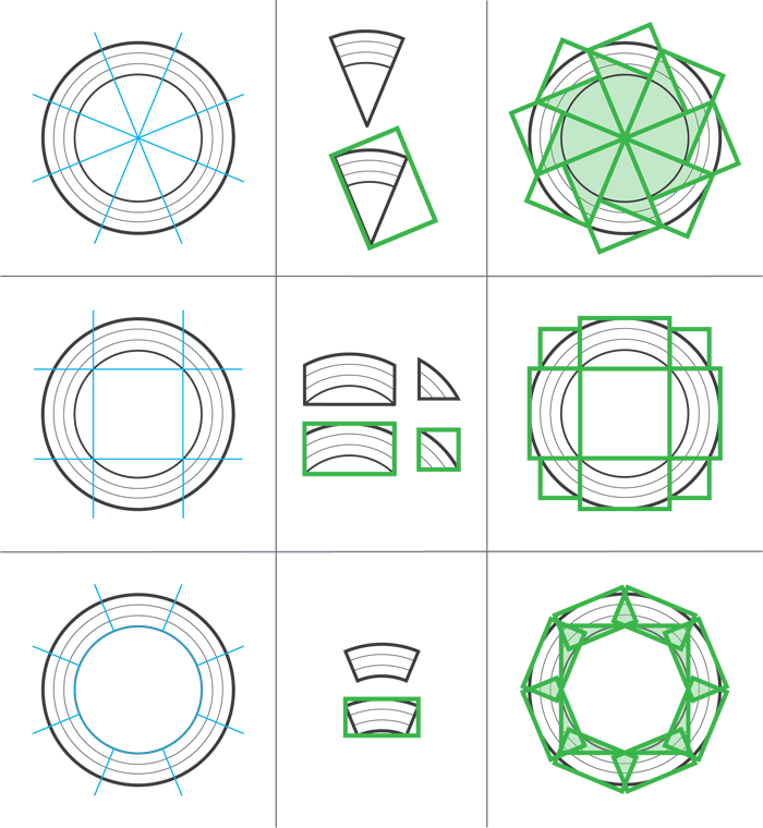
Figure 31: Thought experiment showing how a large model can be cut up and how that affects bounding boxes and their overlap.
Cascaded Shadow Maps
Dynamic Shadow Cascades bring a high level of detail to your game, but they can be expensive and require a powerful gaming PC to run without a loss of frame rate.
Fortunately, as the name suggests, these shadows are dynamically created every frame, so they can be set in-game to allow the player to optimize their preferences.
Cost of Dynamic Shadow Cascades Using Intel HD Graphics 350
The level of Dynamic Shadow Cascades can be dynamically controlled in several ways:
- Shadow quality settings under the Engine Scalability Settings
- Editing the integer value of r.Shadow.CSM.MaxCascades under the BaseScalability.ini file (between 0 and 4) and then changing the sg.ShadowQuality (between 0–3 for Low, Medium, High, and Epic)
- Adding an Execute Console Command node in a blueprint within your game where you manually set the value of r.Shadow.CSM.MaxCascades
Scripting Optimizations
In this part of the tutorial, we go over scripting to help increase the frame rate and stability of a project.
Disabling Fully Transparent Objects
Even fully transparent game objects consume rendering draw calls. To avoid these wasted calls, set the engine to stop rendering them.
To do this with blueprints, UE4 needs multiple systems in place.
Material Parameter Collection
First, create a Material Parameter Collection (MPC). These assets store scalar and vector parameters that can be referenced by any material in the game and can be used to modify those materials during play to allow for dynamic effects.
Create an MPC by selecting it under the Create Advanced Asset > Materials & Textures menu.
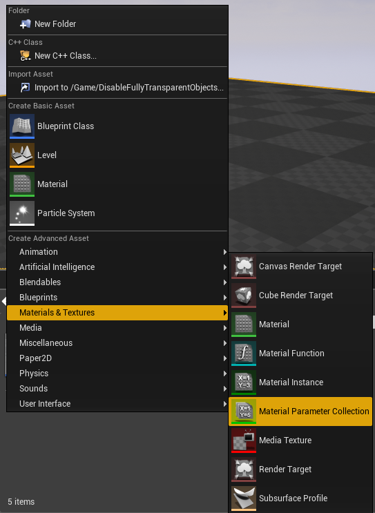
Figure 32: Creating a Material Parameter Collection.
Once in the MPC, default values for scalar and vector parameters can be created, named, and set. For this optimization, we need a scalar parameter that we will call Opacity, and we’ll use it to control the opacity of our material.
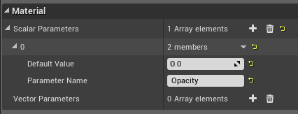
Figure 33: Setting a Scalar Parameter named Opacity.
Material
Next, we need a material to use the MPC. In that material, create a node called Collection Parameter. Through this node, select an MPC and which of its parameters will be used.
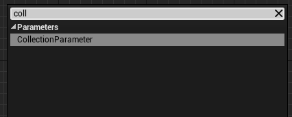
Figure 34: Getting the Collection Parameter node in a material.
Once the node set is created, drag off its return pin to use the value of that parameter.
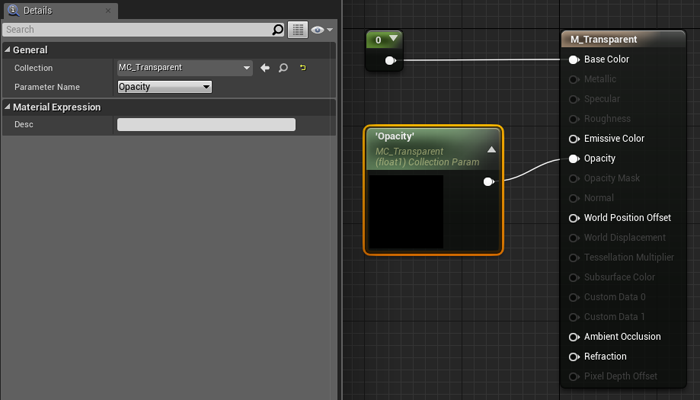
Figure 35: Setting the Collection Parameter in a material.
The Blueprint Scripting Part
After creating the MPC and material, we can set and get the values of the MPC through a blueprint. The values can be called and changed with the Get/Set Scalar Parameter Value and Get/Set Vector Parameter Value. Within those nodes, select the Collection (MPC) to use and a Parameter Name within that collection.
For this example, we set the Opacity scalar value to be the sine of the game time, to see values between 1 and -1.
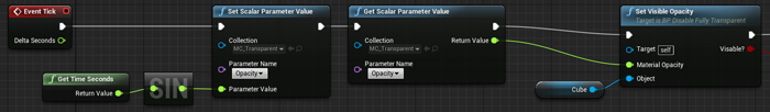
Figure 36: Setting and getting a scalar parameter and using its value in a function.
To set whether the object is being rendered, we create a new function called Set Visible Opacity with an input of the MPC’s Opacity parameter value and a static mesh component, and a Boolean return for whether or not the object is visible.
From that we run a greater than near-zero check, 0.05 in this example. A check of 0 could work, but as zero is approached the player will no longer be able to see the object, so we can turn it off just before it gets to zero. This also helps provide a buffer in the case of floating point errors not setting the scalar parameter to exactly 0, making sure it is turned off if it’s set to 0.0001, for instance.
From there, run a branch where a True condition will Set Visibility of the object to be true, and a False condition to be set to false.
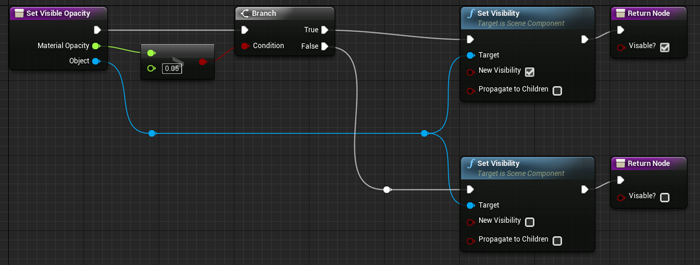
Figure 37: Set Visible Opacity function.
Tick, Culling, and Time
If blueprints within the scene use Event Tick, those scripts are being run even when those objects no longer appear on screen. Normally this is fine, but the fewer blueprints ticking every frame in a scene, the faster it runs.
Some examples of when to use this optimization are:
- Things that do not need to happen when the player is not looking
- Processes that run based on game time
- Non-player characters (NPC) that do not need to do anything when the player is not around
As a simple solution, we can add a Was Recently Rendered check to the beginning of our Event Tick. In this way, we do not have to worry about connecting custom events and listeners to get our tick to turn on and off, and the system can still be independent of other actors within the scene.
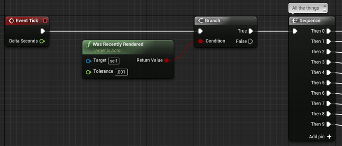
Figure 38: Using the culling system to control the content of Event Tick.
Following that method, if we have a process that runs based on game time, say an emissive material on a button that dims and brightens every second, we use the method that we see in the following figure.
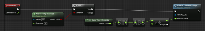
Figure 39: Emissive Value of material collection set to the absolute sine of time when it is rendered.
What we see in the figure is a check of game time that is passed through the absolute value of sine plus one, which gives a sine wave ranging from 1 to 2.
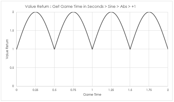
The advantage is that no matter when the player looks at this button, even if they spin in circles or stare, it always appears to be timed correctly to this curve, thanks to the value being based on the sine of game time.
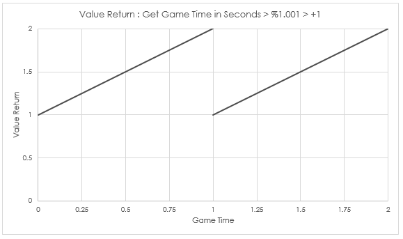
This also works well with modulo, though the graph looks a bit different.
This check can be called later in the Event Tick. If the actor has several important tasks that need to be done every frame, they can be executed before the render check. Any reduction in the number of nodes called on a tick within a blueprint is an improvement.

Figure 40: Using culling to control visual parts of a blueprint.
Another approach to limiting the cost of a blueprint is to slow it down and only let it tick once every time interval. This can be done using the Set Actor Tick Interval node so that the time needed is set through scripting.
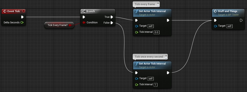
Figure 41: Switching between tick intervals.
In addition, the Tick Interval can be set in the Details tab of the blueprint. This allows setting when the blueprint will tick based on time in seconds.
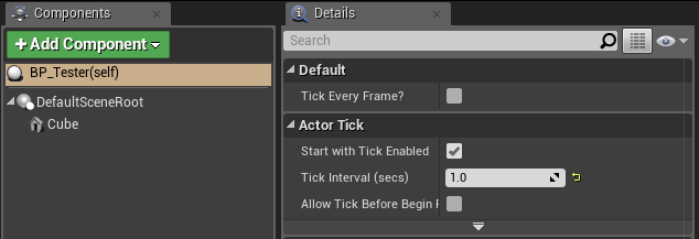
Figure 42: Finding the Tick Interval within the Details tab.
For example, this is useful in the counting of seconds.
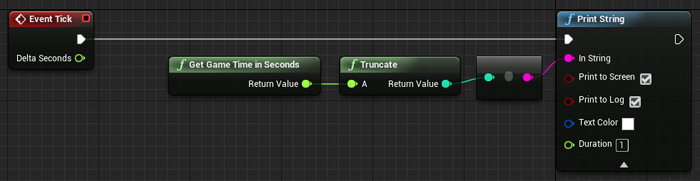
Figure 43: Setting a second counting blueprint to only tick once every second.
As an example of how this optimization could help by reducing the average ms, let’s look at the following example.
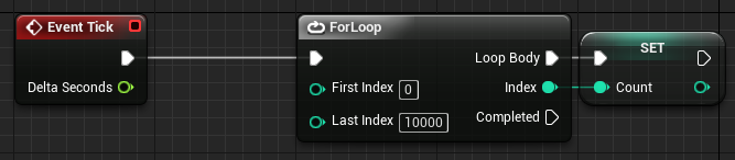
Figure 44: An extremely useful example of something not to do.
Here we have a ForLoop node that counts 0 to 10,000, and we set the integer Count to the current count of the ForLoop. This blueprint is extremely costly and inefficient, so much that it has our scene running at 53.49 ms.
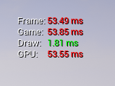
Figure 45: Viewing the cost of the extremely useful example with Stat Unit.
If we go into the Profiler, we see why. This simple yet costly blueprint takes 43 ms per tick.
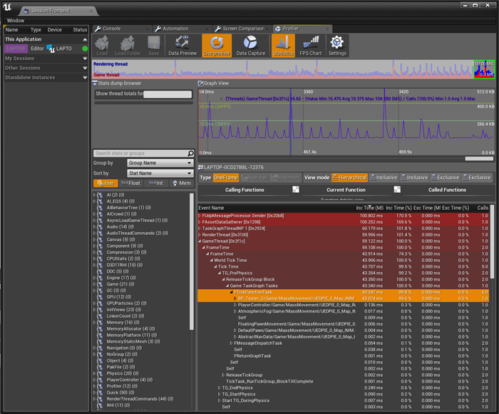
Figure 46: Cost of an extremely useful example ticking every frame as viewed in the Profiler.
However, if we only tick this blueprint once every second, it takes 0 ms most of the time. If we look at the average time (click and drag over an area in the Graph View) over three tick cycles for the blueprint, we see that it uses an average of 0.716 ms.
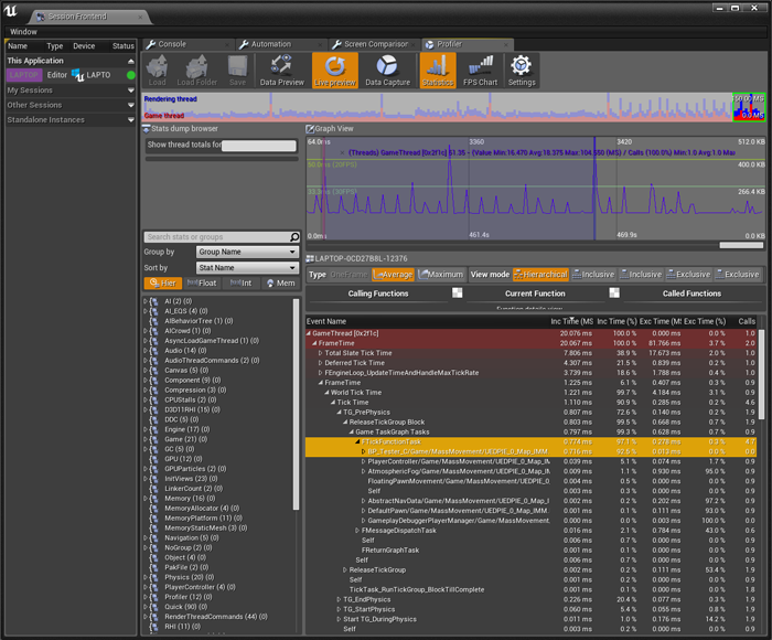
Figure 47: Cost average of the extremely useful example ticking only once every second as viewed in the Profiler.
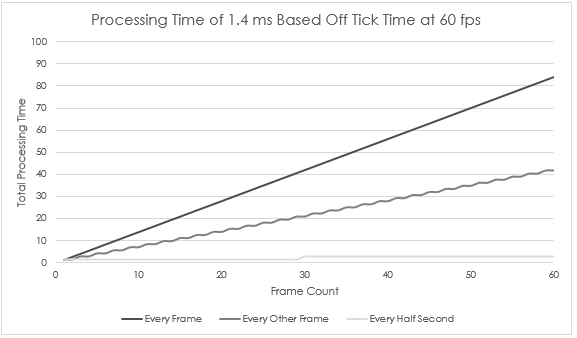
To look at a more common example, if we have a blueprint that runs at 1.4 ms in a scene that is running at 60 fps, it uses 84 ms of processing time. However, if we can reduce its tick time, it reduces the total amount of processing time for the blueprint.
Mass Movement, ForLoops, and Multithreading
The idea of several meshes all moving at once looks awesome and can really sell the visual style of a game. However, the processing cost can put a huge strain on the CPU and, in turn, the fps. Thanks to multithreading and UE4’s handling of worker threads, we can break up the handling of this mass movement across multiple blueprints to optimize performance.
For this section, we will use the following blueprint scripts to dynamically move a collection of 1600 instanced sphere meshes up and down along a modified sine curve.
Here is a simple construction script to build out the grid. Simply add an instanced static mesh component to an actor, choose the mesh to use for it in the Details tab, and then add these nodes to its construction.
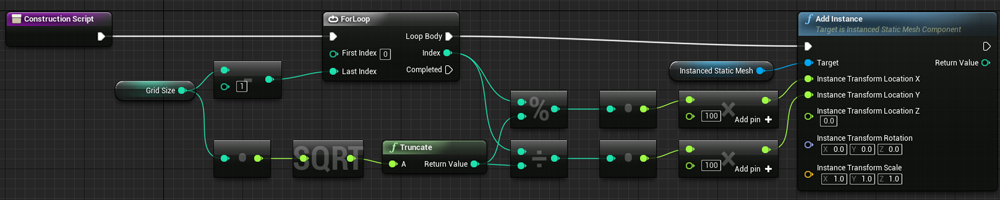
Figure 48: Construction script to build a simple grid.
Once the grid is created, add this blueprint script to the Event Graph.
Something to note about the Update Instance Transform node. When the transform of any instance is modified, the change will not be seen unless Mark Render State Dirty is marked as true. However, it is an expensive operation, as it goes through every mesh in the instance and marks it as dirty. To save on processing, especially if the node is to run multiple times in a single tick, update the meshes at the end of that blueprint. In the script below we Mark Render State Dirty as true only if we are on the Last Index of the ForLoop, if Index is equal to Grid Size minus one.
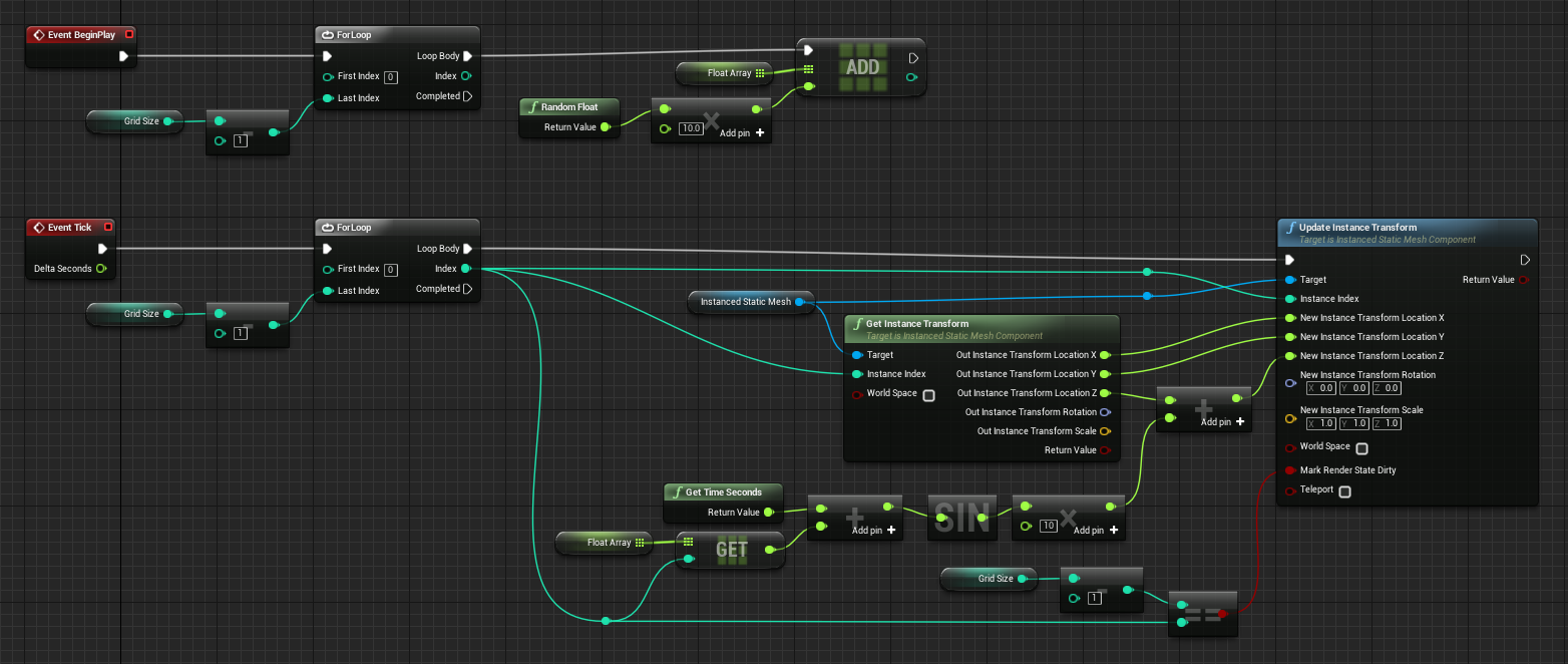
Figure 49: Blueprint for dynamic movement for an instanced static mesh.
With our actor blueprint and the grid creation construction and dynamic movement event we can place several different variants with the goal of always having 1600 meshes displaying at once.
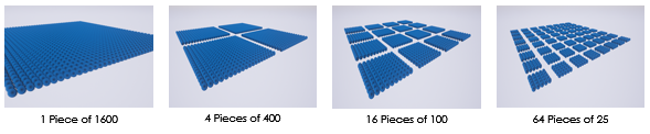
Figure 50: Diagram of the grid of 1600 broken up into different variations.
When we run the scene we get to see the pieces of our grid traveling up and down.
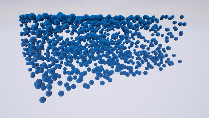
Figure 51: Instanced static mesh grid of 1600 moving dynamically.
However, the breakdown of the pieces we have affects the speed at which our scene runs.
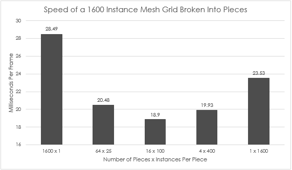
Looking at the chart above, we see that 1600 pieces of one instanced static mesh each (negating the purpose of even using instancing) and the single piece of 1600 run the slowest, while the rest all hover around a performance of 19 and 20 ms.
The reason the individual pieces run the slowest is that the cost of running the 1600 blueprints is 16.86 ms, an average of only 0.0105 ms per blueprint. However, while the cost of each blueprint is tiny, the sheer number of them starts to slow down the system. The only thing that can be done to optimize is to reduce the number of blueprints running per tick. The other slowdown comes from the increased number of draw calls and mesh transform commands caused by the large number of individual meshes.
On the opposite side of the graph, we see the next biggest offender, the single piece of 1600 meshes. This mesh is very efficient on draw calls, since the whole grid is only one draw call, but the cost of running the blueprint that must update all 1600 meshes per tick causes it to take 19.63 ms of time to process.
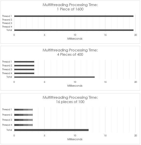
When looking at the processing time for the other three sets, we see the benefits of breaking up these mass-movement actors, thanks to smaller script time and taking advantage of multithreading within the engine. Because UE4 takes advantage of multithreading, it spreads the blueprints across many worker threads, allowing the evaluation to run faster by effectively using all CPU cores.
If we look at a simple breakdown of the processing time for the blueprints and how they are split among the worker threads, we see the following.
Data Structures
Using the correct type of data structure is imperative to any program, and this applies to game development just as much as any other software development. When programming in UE4 with blueprints, no data structures are given for the templated array that will act as the main container. They can be created by hand using functions and the nodes provided by UE4.
Example of Usage
As an example of why and how a data structure could be used in game development, consider a shoot ’em up (Shmup) style game. One of the main mechanics of a Shmup is shooting thousands of bullets across the screen toward incoming enemies. While one could spawn each of the bullets and then destroy them, it would require a lot of garbage collection on the part of the engine, and could cause a slowdown or loss of frame rate. To get around this, developers could consider a spawning pool (collection of objects all placed into an array or list that are processed when the game is started) of bullets, enabling and disabling them as needed, so the engine only needs to create each bullet once.
A common method of using these spawning pools is to grab the first bullet in the array or list not enabled, moving it into a starting position, enabling it, and then disabling it when it flies off-screen or into an enemy. The problem with this method comes from the run time, or Big O, of a script. Because you are iterating through the collection of objects looking for the next disabled object, if the collection is 5,000 objects, for example, it could take up to that many iterations to find one object. This type of function would have a time of O(n), where n is the number of objects in the collection.
While O(n) is far from the worst an algorithm can perform, the closer we can get to O(1), a fixed cost regardless of size, the more efficient our script and game will be. To do this with a spawning pool, we use a data structure called a Queue. Like a queue in real life, this data structure takes the first object in the collection, uses it, and then removes it, continuing the line until every object has been dequeued from the front.
By using a queue for our spawning pool, we can get the front of our collection, enable it, and then pop it (remove it) from the collection and immediately push it (add it) to the back of our collection, creating an efficient cycle within our script and reducing its run time to O(1). We can also add an enabled check to this cycle. If the object that would be popped is enabled, the script would instead spawn a new object, enable it, and then push it to the back of the queue, increasing the size of the collection without decreasing the efficiency of the run time.
Queues
Below is a collection of pictures that illustrate how to implement a queue in blueprints, using functions to help maintain code cleanliness and reusability.
Pop
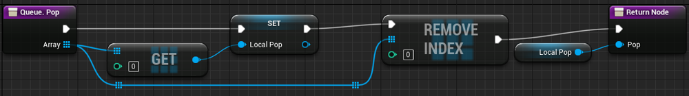
Figure 52: A queue pop with return implemented in blueprints.
Push
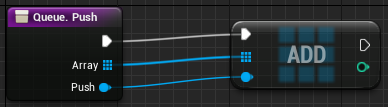
Figure 53: A queue push implemented in blueprints.
Empty
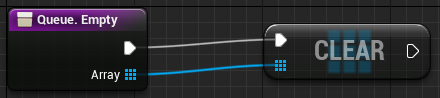
Figure 54: A queue empty implemented in blueprints.
Size
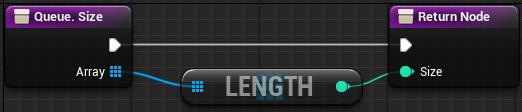
Figure 55: A queue size implemented in blueprints.
Front
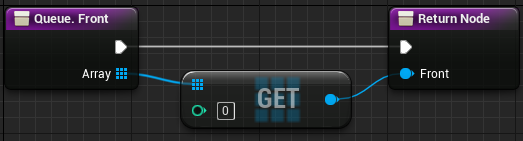
Figure 56: A queue front implemented in blueprints.
Back
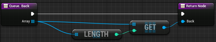
Figure 57: A queue back implemented in blueprints.
Insert
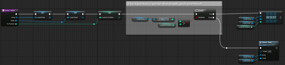
Figure 58: A queue insert with position check implemented in blueprints.
Swap
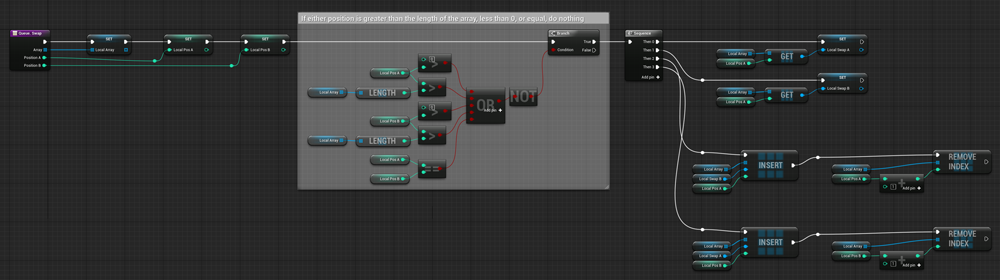
Figure 59: A queue swap with position checks implemented in blueprints.
Stacks
Below is a collection of pictures that illustrate how to implement a stack in blueprints, using functions to help maintain code cleanliness and reusability.
Pop
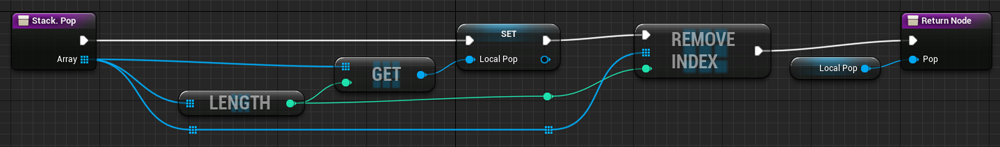
Figure 60: A stack pop with return implemented in blueprints.
Push
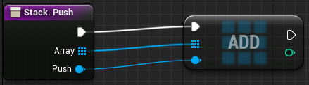
Figure 61: A stack push implemented in blueprints.
Empty
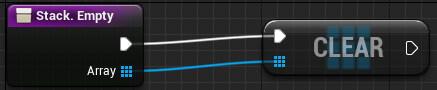
Figure 62: A stack empty implemented in blueprints.
Size
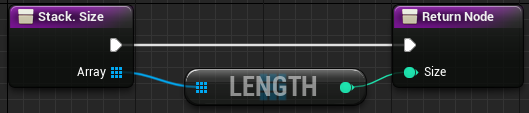
Figure 63: A stack size implemented in blueprints.
Back
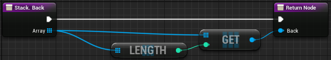
Figure 64: A stack back implemented in blueprints.
Insert
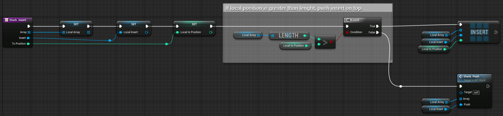
Figure 65: A stack insert with position check implemented in blueprints.
Optimization Viewmodes
You can change the way in which the scene is rendered when editing the project by changing the viewmode within the scene view port. Under this tab is the Optimization Viewmodes section; each of these views will help to identify certain optimizations that you can make. We will go over them in the order that they appear.
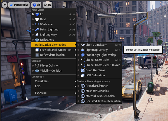
Figure 66: Finding the selection of optimization viewmodes.
This documentation doesn’t cover the Texture Streaming Accuracy portion of the Optimization Viewmodes, as they are more relevant to the creation of 3D models, but for information on what they show, see the Epic Games documentation on texture streaming.
Light Complexity
The Light Complexity view shows us how our scene is being lit by our lights, the influence area of those lights, and how much cost to performance they can infer throughout the scene.
When we add a point light to the center of the scene, we can see the influence this light has on the complexity of the lighting in the scene.
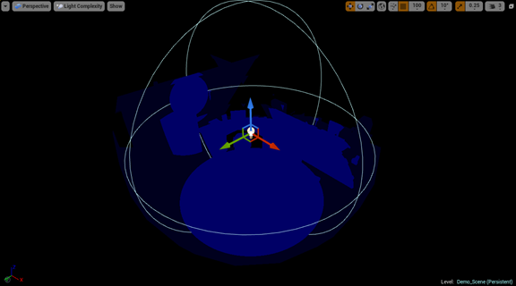
Figure 67: Single point light complexity.
If we create more point lights in the same area, we begin to see the cost of the overlapping through the visualizer. As more and more lights begin to overlap, the influenced areas will become red, then white.
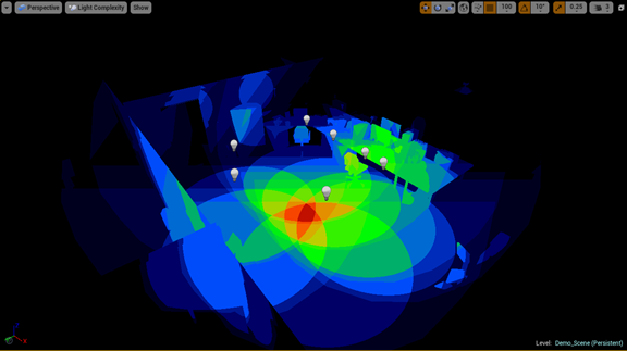
Figure 68: Light complexity of multiple point light sources.
The performance hit comes from each pixel in the overlap needing to be shaded by multiple sources. The cost of this on static lights is primarily a hit on the time it takes to bake the lighting of the scene, but when using movable or stationary lighting, the cost of dynamic lighting and shadows is increased.
To reduce the impact on scene performance, lights that cause overlap should be removed, switched to static, or their position and influence should be adjusted.
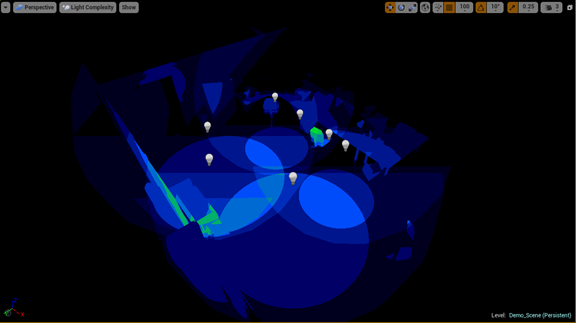
Figure 69: Lesser complexity by adjusting light radius.
Lightmap Density
The density of the lightmap for objects in your scene shows the texel density of the lighting effects that will be placed on those objects. For the viewport visuals, the greener the color-coded shade, the better the texel density of the lightmap for the object; while blue is less dense and red is denser. Because each lightmap is a texture, your texture streaming budget can be quickly used up if the number of objects in your scene goes up, or you use higher lightmap resolutions to increase the visual fidelity of the render.
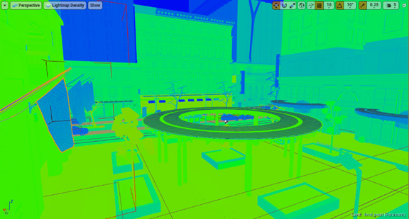
Figure 70: Scene view of lightmap density.
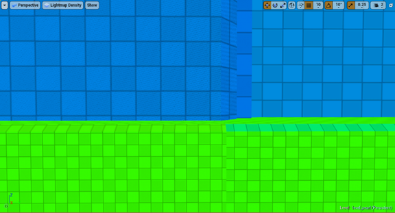
Figure 71: Up close view of different lightmap densities.
To change the lightmap density for any object in your scene, adjust the Overridden Light Map Resolution value (default of 64) to another value that better fits the texel density of that object. As with other textures, sticking to powers of two (2, 4, 8, 16, 32, 64, and so on) will reduce wasted rendering.
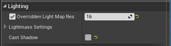
Figure 72: Overridden Light Map Resolution.
Below, we can see a streetlight in the scene with the default lightmap resolution of 64. When its value is switched to 16, we see its color change from red to green; a better density and cheaper lightmap for streaming.
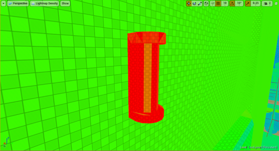
Figure 73: Object with a dense lightmap.
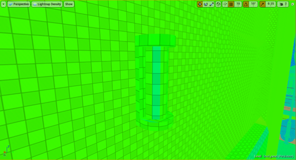
Figure 74: Same object with an optimal lightmap density.
Stationary Light Overlap
In the Unreal Engine (UE), the stationary light plays a unique role in the development process. However, there is a limit to the number of stationary lights that may overlap, and going over that limit causes a hit on performance.
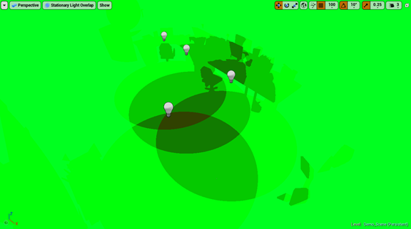
Figure 75: Collection of stationary lights and their overlaps.
When more than four stationary lights overlap, any additional stationary lights are forced to work as movable lights, increasing the performance requirement of each additional light. If we switch all the lights to be stationary, we can see their influence over each other. The lighter the green, the fewer overlaps.
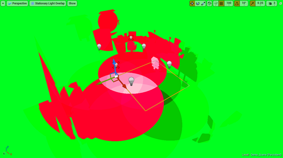
Figure 76: Stationary lights with too many overlaps.
After four overlaps, the color changes to red. Any light involved in the red overlap will be rendered as a movable light, displayed as a red X over the light’s billboard. To fix this issue, some of the offending lights must be removed, switched to static, or have their influence area reduced or moved.
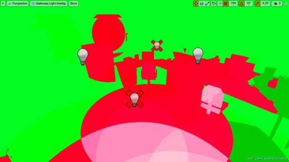
Figure 77: Stationary lights crossed out, showing that they will be used as movable lights instead.
Shader Complexity (and Quads)
This view allows you to see the number of shaders being calculated per pixel in your current view, with green being the lowest and red and white being the highest (most expensive).
If we look at Robo Recall*, we see that the shader complexity of the whole scene is relatively light, with most of the cost going into the street around the city. Epic Games made a large effort to reduce their shader complex to help hit their 90 fps goal for the VR title.
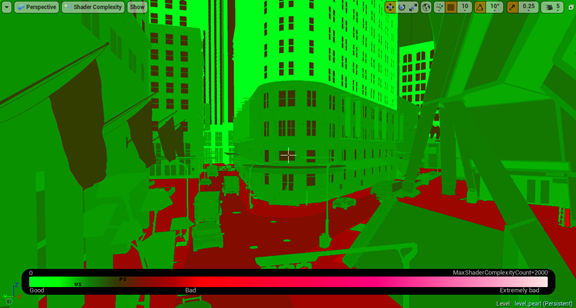
Figure 78: View of a scene with an optimized shader.
However, looking at a forest scene, we see that the shader complexity of the trees and their leaves is ridiculously high and unoptimized.
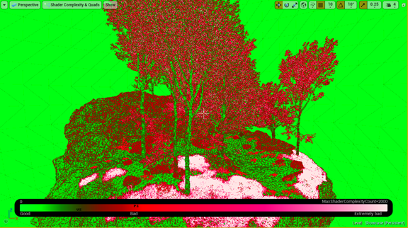
Figure 79: View of a scene with a large number of complex shaders.
To reduce the complexity of your shaders, the number of materials and the number of texture lookups within those materials needs to be reduced.
In addition, one of the biggest hits to performance with shader complexity comes from opacity, a main component of foliage and particle systems, and the reason the trees have such a high complexity.
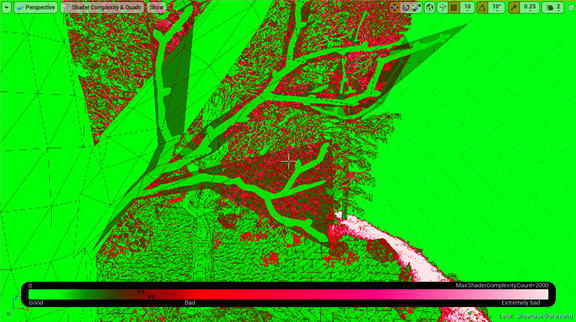
Figure 80: Up close view of how transparencies affect shader complexity.
To reduce the number of opacity materials in your scene, you can design around it (Robo Recall has trees that are solar panel towers shaped to look like trees) or use LOD for your foliage and particles to reduce the number of meshes with opacity at a distance, a problem that unfortunately needs to be thought about early in development or made up for with model production later in the project’s timeline.
Quad Overdraw
When multiple polygons are all overlapping and being rendered within the same quad on the graphics processing unit, the performance of the scene will suffer as these renders are calculated and then unused.
This issue is caused by the complexity of the meshes and the distance they are from the camera; the smaller the visible triangles of a mesh, the more are within a quad. If we look at the two pictures, we see Robo Recall with some overdraw on the edges of models and, at a distance, our forest scene where there is a large amount of overdraw occurring within the trees around the whole forest. As with shader complexity, opacity is a major performance hit and causes a lot of overdraw.
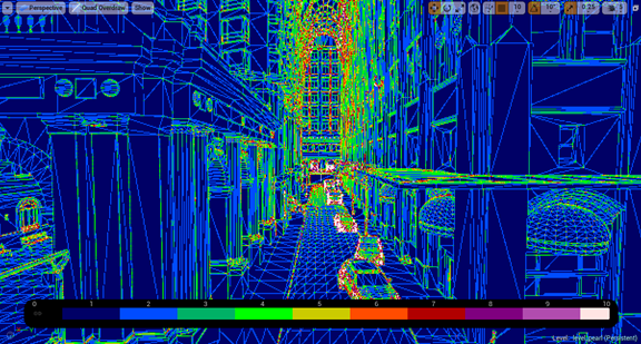
Figure 81: Scene view of quad-overdraw.

Figure 82: Scene view of a large amount of quad-overdraw.
To reduce the amount of overdraw, use LODs to reduce the poly count of models at a distance and reduce transparencies in particle systems and foliage.
LOD Coloration
Knowing when your LODs switch is important for the visuals of your game, and the LOD coloration view gives you that information. LODs are crucial to optimizing any title, as they save on rendering details that cannot be seen from a distance and the triangle count of your models. Along with what was previously mentioned, LODs also help with quad overdraw and shader complexity performance issues.
Adding LODs can be done with modeling software or by using auto LOD generation (UE 4.12+), and the switch distance can be adjusted to work for your scene.
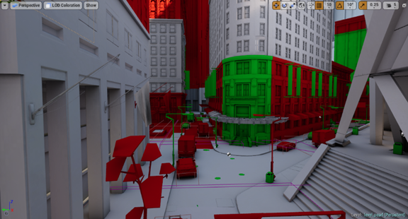
Figure 83: Scene view of level of details.
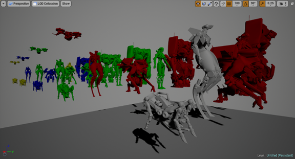
Figure 84: Skeletal mesh lineup of LODs.