Unreal* Engine 4 Optimization Tutorial, Part 3

The contents of this guide work for version 4.19 of the Unreal Engine.

This is part 3 of a tutorial to help developers improve the performance of their games in Unreal Engine* 4 (UE4). In this tutorial, we go over a collection of tools to use within and outside of the engine, as well some best practices for the editor, and scripting to help increase the frame rate and stability of a project.

Scripting Optimizations

Disabling Fully Transparent Objects

Even fully transparent game objects consume rendering draw calls. To avoid these wasted calls, set the engine to stop rendering them.

To do this with Blueprints, UE4 needs multiple systems in place.

Material Parameter Collection

First, create a Material Parameter Collection (MPC). These assets store scalar and vector parameters that can be referenced by any material in the game, and can be used to modify those materials during play to allow for dynamic effects.

Create an MPC by selecting it under the Create Advanced Asset > Materials & Textures menu.

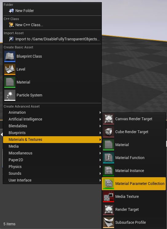
Figure 32: Creating a Material Parameter Collection.

Once in the MPC, default values for scalar and vector parameters can be created, named and set. For this optimization, we need a scalar parameter that we will call Opacity and we’ll use it to control the opacity of our material.

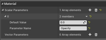
Figure 33: Setting a Scalar Parameter named Opacity.

Material

Next, we need a material to use the MPC. In that material, create a node called Collection Parameter. Through this node, select an MPC and which of its parameters will be used.

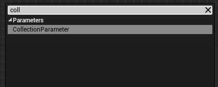
Figure 34: Getting the Collection Parameter node in a material.

Once the node set is created, drag off its return pin to use the value of that parameter.

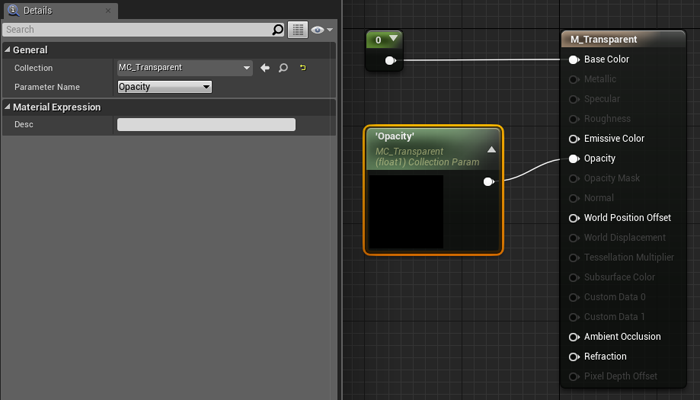
Figure 35: Setting the Collection Parameter in a material.

The Blueprint Scripting Part

After creating the MPC and material we can set and get the values of the MPC through a blueprint. The values can be called and changed with the Get/Set Scalar Parameter Value and Get/Set Vector Parameter Value. Within those nodes, select the Collection (MPC) to use and a Parameter Name within that collection.

For this example, we set the Opacity scalar value to be the sine of the game time, to see values between 1 and -1.

Figure 36: Setting and getting a scalar parameter and using its value in a function.

To set whether the object is being rendered, we create a new function called Set Visible Opacity with an input of the MPC’s Opacity parameter value and a static mesh component, and a Boolean return for whether or not the object is visible.

From that we run a greater than near-zero check, 0.05 in this example. A check of 0 could work, but as zero is approached the player will no longer be able to see the object, so we can turn it off just before it gets to zero. This also helps provide a buffer in the case of floating point errors not setting the scalar parameter to exactly 0, making sure it is turned off if it’s set to 0.0001, for instance.

From there, run a branch where a True condition will Set Visibility of the object to be true, and a False condition to be set to false.

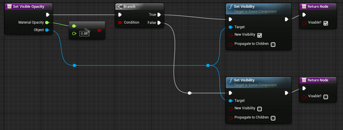
Figure 37: Set Visible Opacity function.

Tick, Culling, and Time

If blueprints within the scene use Event Tick, those scripts are being run even when those objects no longer appear on screen. Normally this is fine, but the fewer blueprints ticking every frame in a scene, the faster it runs.

Some examples of when to use this optimization are:

Things that do not need to happen when the player is not looking
Processes that run based on game time
Non-Player Characters (NPC) that do not need to do anything when the player is not around

As a simple solution, we can add a Was Recently Rendered check to the beginning of our Event Tick. In this way, we do not have to worry about connecting on custom events and listeners to get our tick to turn on and off, and the system can still be independent of other actors within the scene.

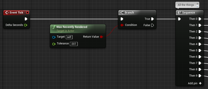
Figure 38: Using the culling system to control the content of Event Tick.

Following that method, if we have a process that runs based on game time, say an emissive material on a button that dims and brightens every second, we use the method that we see below.

Figure 39: Emissive Value of material collection set to the absolute sine of time when it is rendered.

What we see in the figure is a check of game time that is passed through the absolute value of sine plus one, which gives a sine wave ranging from 1 to 2.

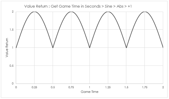
The advantage is that no matter when the player looks at this button, even if they spin in circles or stare, it always appears to be timed correctly to this curve thanks to the value being based on the sine of game time.

This also works well with modulo, though the graph looks a bit different.

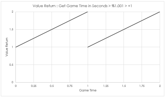
This check can be called later into the Event Tick. If the actor has several important tasks that need to be done every frame, they can be executed before the render check. Any reduction in the number of nodes called on a tick within a blueprint is an improvement.

Figure 40: Using culling to control visual parts of a blueprint.

Another approach to limiting the cost of a blueprint is to slow it down and only let it tick once every time interval. This can be done using the Set Actor Tick Interval node so that the time needed is set through scripting.

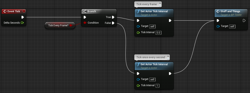
Figure 41: Switching between tick intervals.

In addition, the Tick Interval can be set in the Details tab of the blueprint. This allows setting when the blueprint will tick based on time in seconds.

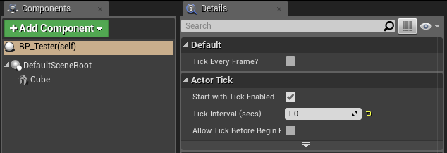
Figure 42: Finding the Tick Interval within the Details tab.

For example, this is useful in the counting of seconds.

Figure 43: Setting a second counting blueprint to only tick once every second.

As an example of how this optimization could help by reducing the average ms, let’s look at the following example.

Figure 44: An extremely useful example of something not to do.

Here we have a ForLoop node that counts 0 to 10000, and we set the integer Count to the current count of the ForLoop. This blueprint is extremely costly and inefficient, so much that it has our scene running at 53.49 ms.

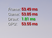
Figure 45: Viewing the cost of the extremely useful example with Stat Unit.

If we go into the Profiler we see why. This simple yet costly blueprint takes 43 ms per tick.

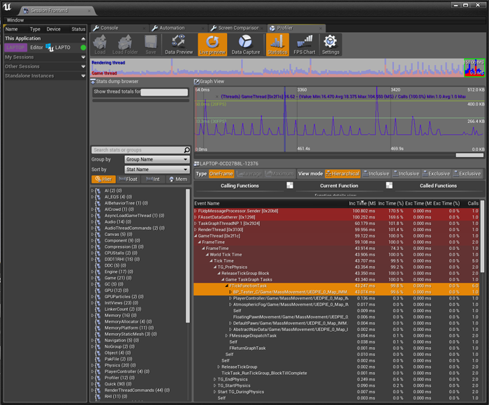
Figure 46: Cost of extremely useful example ticking every frame as viewed in the Profiler.

However, if we only tick this blueprint once every second, it takes 0 ms most the time. If we look at the average time (click and drag over an area in the Graph View) over three tick cycles for the blueprint we see that it uses an average of 0.716 ms.

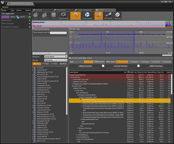
Figure 47: Cost average of the extremely useful example ticking only once every second as viewed in the Profiler.

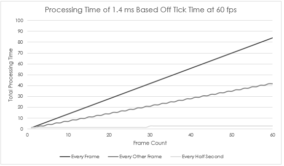
To look at a more common example, if we have a blueprint that runs at 1.4 ms in a scene that is running at 60 fps, it uses 84 ms of processing time. However, if we can reduce its tick time, it reduces the total amount of processing time for the blueprint.

Mass Movement, ForLoops, and Multithreading

The idea of several meshes all moving at once looks awesome and can really sell the visual style of a game. However, the processing cost can put a huge strain on the CPU and, in turn, the FPS. Thanks to multithreading and UE4’s handling of worker threads, we can break up the handling of this mass movement across multiple blueprints to optimize performance.

For this section, we will use the following blueprint scripts to dynamically move a collection of 1600 instanced sphere meshes up and down along a modified sine curve.

Here is a simple construction script to build out the grid. Simply add an Instanced Static Mesh component to an actor, choose the mesh to use for it in the Details tab, and then add these nodes to its construction.

Figure 48: Construction Script to build a simple grid.

Once the grid is created, add this blueprint script to the Event Graph.

Something to note about the Update Instance Transform node. When the transform of any instance is modified, the change will not be seen unless Mark Render State Dirty is marked as true. However, it is an expensive operation, as it goes through every mesh in the instance and marks it as dirty. To save on processing, especially if the node is to run multiple times in a single tick, update the meshes at the end of that blueprint. In the script below we Mark Render State Dirty as true only if we are on the Last Index of the ForLoop, if Index is equal to Grid Size minus one.

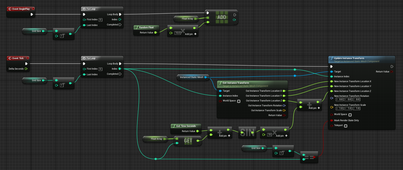
Figure 49: Blueprint for dynamic movement for an instanced static mesh.

With our actor blueprint and the grid creation construction and dynamic movement event we can place several different variants with the goal of always having 1600 meshes displaying at once.

Figure 50: Diagram of the grid of 1600 broken up into different variations.

When we run the scene we get to see the pieces of our grid traveling up and down.

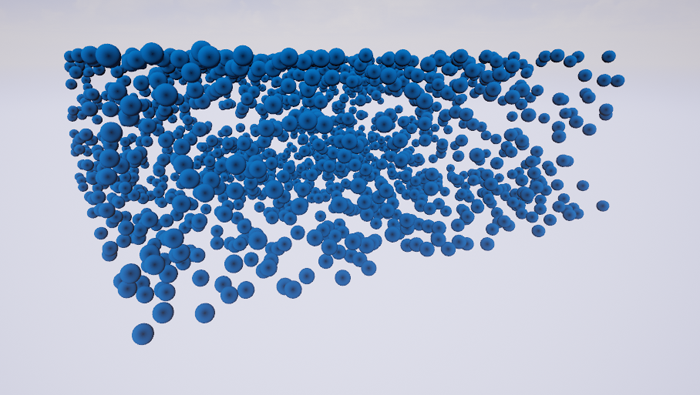
Figure 51: Instanced static mesh grid of 1600 moving dynamically.

However, the breakdown of the pieces we have affects the speed at which our scene runs.

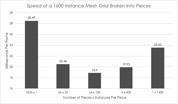
Looking at the chart above, we see that 1600 pieces of one Instanced Static Mesh each (negating the purpose of even using instancing) and the single piece of 1600 run the slowest, while the rest all hover around a performance of 19 and 20 ms.

The reason the individual pieces runs the slowest is that the cost of running the 1600 blueprints is 16.86 ms, an average of only 0.0105 ms per blueprint. However, while the cost of each blueprint is tiny, the sheer number of them starts to slow down the system. The only thing that can be done to optimize is to reduce the number of blueprints running per tick. The other slowdown comes from the increased number of draw calls and mesh transform commands caused by the large number of individual meshes.

On the opposite side of the graph we see the next biggest offender, the single piece of 1600 meshes. This mesh is very efficient on draw calls, since the whole grid is only one draw call, but the cost of running the blueprint that must update all 1600 meshes per tick causes it to take 19.63 ms of time to process.

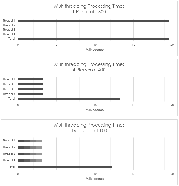
When looking at the processing time for the other three sets we see the benefits of breaking up these mass-movement actors, thanks to smaller script time and taking advantage of multithreading within the engine. Because UE4 takes advantage of multithreading, it spreads the blueprints across many worker threads, allowing the evaluation to run faster by effectively utilizing all CPU cores.

If we look at a simple breakdown of the processing time for the blueprints and how they are split among the worker threads, we see the following.

Data Structures

Using the correct type of Data Structure is imperative to any program, and this applies to game development just as much as any other software development. When programming in UE4 with blueprints, no data structures are given for the templated array that will act as the main container. They can be created them by hand using functions and the nodes provided by UE4.

Example of Usage

As an example of why and how a data structure could be used in game development, consider a shoot ’em up (Shmup) style game. One of the main mechanics of a Shmup is shooting thousands of bullets across the screen toward incoming enemies. While one could spawn each of the bullets and then destroy them, it would require a lot of garbage collection on the part of the engine, and could cause a slowdown or loss of frame rate. To get around this, developers could consider a spawning pool (collection of objects all placed into an array or list which are processed when the game is started) of bullets, enabling and disabling them as needed, so the engine only needs to create each bullet once.

A common method of using these spawning pools is to grab the first bullet in the array/list not enabled, moving it into a starting position, enabling it, and then disabling it when it flies off screen or into an enemy. The problem with this method comes from the run time, or Big O, of a script. Because you are iterating through the collection of objects looking for the next disabled object, if the collection is 5000 objects for example, it could take up to that many iterations to find one object. This type of function would have a time of O(n), where n is the number of objects in the collection.

While O(n) is far from the worst an algorithm can perform, the closer we can get to O(1), a fixed cost regardless of size, the more efficient our script and game will be. To do this with a spawning pool we use a data structure called a Queue. Like a queue in real life, this data structure takes the first object in the collection, uses it, and then removes it, continuing the line until every object has been de-queued from the front.

By using a queue for our spawning pool, we can get the front of our collection, enable it, and then pop it (remove it) from the collection and immediately push it (add it) to the back of our collection; creating an efficient cycle within our script and reducing its run time to O(1). We can also add an enabled check to this cycle. If the object that would be popped is enabled, the script would instead spawn a new object, enable it, and then push it to the back of the queue, increasing the size of the collection without decreasing the efficiency of the run time.

Queues

Below is a collection of pictures that illustrate how to implement a queue in blueprints, using functions to help maintain code cleanliness and reusability.

Pop

Figure 52: A queue pop with return implemented in blueprints.

Push

Figure 53: A queue push implemented in blueprints.

Empty

Figure 54: A queue empty implemented in blueprints.

Size

Figure 55: A queue size implemented in blueprints.

Front

Figure 56: A queue front implemented in blueprints.

Back

Figure 57: A queue back implemented in blueprints.

Insert

Figure 58: A queue insert with position check implemented in blueprints.

Swap

Figure 59: A queue swap with position checks implemented in blueprints.

Stacks

Below is a collection of pictures that illustrate how to implement a stack in blueprints, using functions to help maintain code cleanliness and reusability.

Pop

Figure 60: A stack pop with return implemented in blueprints.