One of the key challenges in large language model (LLM) training is reducing the memory requirements needed for training without sacrificing compute and communication efficiency and model accuracy.
Microsoft DeepSpeed* is a popular deep learning software library that facilitates memory-efficient training of LLMs. DeepSpeed includes Zero Redundancy Optimizer (ZeRO), a memory-efficient approach for distributed training. ZeRO has multiple stages of memory-efficient optimizations, and Intel® Gaudi® software currently supports ZeRO-1 and ZeRO-2.
In this article, we talk about what ZeRO is and how it is useful for training LLMs. We provide a brief technical overview of ZeRO, covering the ZeRO-1 and ZeRO-2 stages of memory optimization. Now, we dive into why we need memory-efficient training for LLMs and how ZeRO can help achieve this.
Emergence of LLMs
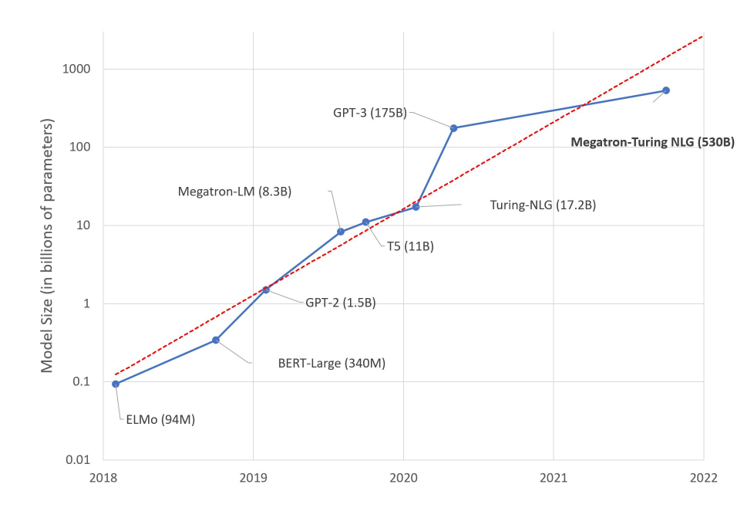
LLMs are becoming super large, with model sizes growing by 10x in only a few years, as shown in Figure 1. An increase in model sizes offers considerable gains in model accuracy. LLMs such as GPT-2* (1.5 B), Megatron-LM (8.3 B), T5 (11 B), Turing-NLG (17 B), Chinchilla (70 B), GPT-3* (175 B), OPT-1 (75 B), and BLOOM (176 B) have been released to excel in various tasks such as natural language understanding, question answering, summarization, translation, and natural language generation. As the size of LLMs keeps growing, how can we efficiently train such large models? The answer is parallelization.
Parallelize Model Training
Data parallelism (DP) and model parallelism are two known techniques in distributed training. In data-parallel training, each data-parallel process or worker has a copy of the complete model, but the dataset is split into Nd parts where Nd is the number of data-parallel processes. If you have Nd devices, split a minibatch into Nd parts, one for each of them. Then feed the respective batch through the model on each device and obtain gradients for each split of the minibatch. Then collect all the gradients and update the parameters with the overall average. Calculate the average of the gradients and use the average of the gradients to update the model and parameters. Then move on to the next iteration of model training. The degree of DP is the number of splits and is denoted by Nd.
With model parallelism, instead of partitioning the data, we divide the model into Nm parts, typically where Nm is the number of devices. Splitting the model can happen either vertically or horizontally. Intra-layer model parallelism is vertical splitting, where each model layer can split across multiple devices. Inter-layer model parallelism (also known as pipeline parallelism) is horizontal splitting, where the model is split at one or more model layer boundaries. Model parallelism requires considerable communication overhead, so it is effective inside a single node but has scaling issues across nodes to communication overheads. Also, it is complex to implement.
Data-parallel training is simpler to implement and has good compute and communication efficiency, but it does not reduce the memory footprint across a single device since the full copy of the model is kept on each device. As models keep growing, it may no longer be possible to hold the full model in a single device’s memory. Typically models with more than approximately 1 B parameters may run out of memory on first-generation Intel® Gaudi® processors that have only 32 GB of high-bandwidth memory (HBM). Second-generation Intel Gaudi 2 processors that have 96 GB of HBM can fit much larger models fully in memory. However, as model sizes keep growing exponentially to 500 B parameters and higher, memory footprint becomes the main bottleneck in model training. So how do we reduce the memory footprint so we can support data-parallel training of large models? To answer that question, we need to know what constitutes the major memory overheads in training large models on hardware for deep learning. So, let's look at this point first.
Where Did All My Memory Go?
The major consumers of memory are model states. Model states include the tensors representing the optimizer states, gradients, and parameters. The second consumers of memory are residual states, which include activations, temporary buffers, and unusable fragmented memory. There are two key observations to note regarding memory consumption during training:
- Model states often consume the largest amount of memory during training. Data-parallel training replicates all model states across all data-parallel processes. This leads to redundant memory consumption.
- We maintain all the required model states statically throughout the entire training process, even though not all model states are required at all times during the training.
These observations lead us to consider how we can reduce redundant memory consumption due to the replication of model states and maintain only needed values during different stages of a training iteration.
Why do model states need so much memory? One of the culprits is the optimizer states. Let us look at Adam, a popular optimizer used for deep learning training. Adam is an extension of the standard stochastic gradient descent algorithm. The Adam optimizer adapts the learning rates based on the average first moment of the gradients (the mean) and the average of the second moments of the gradients (the uncentered variance). Therefore, it needs to store the two optimizer states for each parameter, namely the time-averaged momentum and the variance of the gradients to compute the parameter updates. In addition, the memory requirement is exacerbated further when deploying mixed precision training, as we discuss next.
The state-of-the-art approach to train large models is through mixed precision (bfloat16 and FP32) training, where parameters and activations are stored as bfloat16. During mixed-precision training, both the forward and backward propagation are performed using BF16 weights and activations. However, to effectively compute and apply the updates at the end of the backward propagation, the mixed-precision optimizer keeps an FP32 copy of all the optimizer states that include an FP32 copy of the parameters and other optimizer states. Once the optimizer updates are done, BF16 model parameters are updated from this optimizer copy of FP32 parameters.
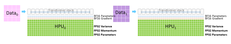
Both Intel Gaudi 2 processors and first-generation Intel Gaudi processors support the BF16 data type. As in Figure 2, which shows a data-parallel training setup with two data-parallel units, we need to have memory for holding the following:
- BF16 parameters
- BF16 gradients
- FP32 optimizer states, which include FP32 momentum of the gradients, FP32 variance of the gradients, and FP32 parameters
For instance, let's consider a model with N parameters, trained using an Adam optimizer with mixed-precision training. We need 2N bytes for bfloat16 parameters and 2N bytes for bfloat16 gradients. For the optimizer states, we need 4N bytes for FP32 parameters, 4N bytes for the variance of the gradients, and 4N bytes for the momentum of the gradients, so the optimizer states require a total of 12N bytes of memory. While our example optimizer was Adam, different optimizers would have different degrees of extra memory states needed. To generalize the memory requirements associated with optimizer states, we denote it as KN, where N is the number of model parameters and K is an optimizer-specific constant. For the Adam optimizer, K is 12.
Considering a model with 1 billion parameters, optimizer states consume 12 GB, which is huge compared to the 2 GB of memory needed for storing bfloat16 model parameter weights. Recall that in standard data-parallel training, each data-parallel process needs to keep a copy of the complete model, including model weights, gradients, and optimizer states. This means that we end up having redundant copies of optimizer states at each DP process, with each occupying 12 GB of memory for 1 billion parameters.
Now that we know that optimizer states occupy a huge redundant memory overhead, how do we optimize away this overhead? This is where DeepSpeed ZeRO kicks in, which is discussed next.
ZeRO Memory-Efficient Optimizations
As we discussed, standard data-parallel training results in redundant memory occupancy of model states at each data-parallel process. ZeRO eliminates this memory redundancy by partitioning the model states across the data-parallel processes. ZeRO consists of multiple stages of memory optimizations depending on the degree of partitioning of model states. ZeRO-1 partitions only the optimizer states. ZeRO-2 partitions both the optimizer states and the gradients. ZeRO-3 partitions all three model states—namely, optimizer states, gradients, and parameters—across the data-parallel processes. Since Intel Gaudi software supports the DeepSpeed ZeRO-2 stage, it enables the partitioning of both optimizer states and gradients.
ZeRO-1 stage is all about partitioning the optimizer states alone across the data-parallel processes. Given a DP training setup of degree Nd, group the optimizer states into Nd equal partitions such that the ith data-parallel process only updates the optimizer states corresponding to the ith partition. This means that each data-parallel process only needs to store and update 1/Nd of the total optimizer states. At the end of each training step, an all-gather across the data-parallel processes is performed to get the fully updated parameters across all data-parallel processes. Since each data-parallel process is concerned with storing and updating 1/Nd of the total optimizer states, it also needs to update only 1/Nd of the total parameters, hence each data-parallel process now has memory requirements for optimizer states cut down to 1/Nd of the earlier requirements. If the original memory requirement of the standard DP setup is 4N + KN, where K is the memory constant associated with the optimizer and N is the number of model parameters, ZeRO stage 1 reduces the memory requirements to 2N + 2N + (KN)/Nd. For a sufficiently high degree of Nd, this can be approximated to 4N. Considering a model with 1 billion parameters and the Adam optimizer where K is 12, standard DP consumes 16 GB of memory for model states, whereas with ZeRO stage 1, this reduces to 4 GB, resulting in a reduction of memory overheads by 4X.
ZeRO-2 stage partitions both the optimizer states and gradients across the data-parallel processes. Recall the fact that each data-parallel process updates only the parameters corresponding to each partition. This means that each data-parallel process needs only the gradients corresponding to that partition and not all the gradients. As gradients of different layers become available during back-propagation, we reduce these gradients only on the data-parallel process corresponding to the relevant parameter partition. In standard DP, this would have been an all-reduce operation, but now it is a reduced operation per data-parallel process. After the reduction operation is done, the gradients are no longer needed and the memory can be released. This reduces the memory required for gradients from 2N in standard DP to 2N/Nd with ZeRO stage 2.
By applying just the optimizer state partition, we have the memory requirements of training an N parameter model to 2N (parameters) + 2N (gradients) + KN/Nd (optimizer states). Now with both optimizer and gradients partitioning in ZeRO stage 2, this reduces to 2N + 2N/Nd + KN/Nd. For the Adam optimizer, this becomes 2N + 14N/Nd. For a sufficiently large Nd, this approximates to 2N. For training a model with 1 billion parameters with the Adam optimizer, standard DP requires 16 GB for model states, whereas with ZeRO stage 2, it becomes 2 GB, resulting in a memory reduction of 8x.
DeepSpeed ZeRO-2 Is Available on Intel Gaudi Software
Support for memory-efficient optimizations enables effective training of large models on the Intel Gaudi platform. DeepSpeed ZeRO-2 is available on the Intel Gaudi software release. Use the Intel Gaudi software fork of the DeepSpeed library, which includes changes to add support for Intel Gaudi processors. For more information, see the DeepSpeed User Guide. The GitHub* page for Intel Gaudi software has examples of training 1.5 B and 5 B parameter BERT models on Intel Gaudi processors using DeepSpeed ZeRO-1 and ZeRO-2.
References
- ZeRO and DeepSpeed: New System Optimizations Enable Training Models with over 100 Billion Parameters
- ZeRO-2 and DeepSpeed: Shatter Barriers of Deep Learning Speed & Scale
- ZeRO: Memory Optimizations Toward Training Trillion Parameter Models
- DeepSpeed User Guide
- Use DeepSpeed and Megatron to Train Megatron-Turing NLG 530B