Accelerate NPU-Bound AI PC Applications using Intel® VTune™ Profiler on Intel® Core™ Ultra Processor

Intel Core Ultra processors consist of three important compute engines to deliver industry-leading end-user experience.   Each of these three compute engines is central to accelerating AI workloads. The Neural Processing Unit (NPU) is an AI accelerator integrated into Intel Core Ultra processors, characterized by a unique architecture comprising compute acceleration and data transfer capabilities. Its compute acceleration is facilitated by Neural Compute Engines, which consist of hardware acceleration blocks for AI operation.

NPUs are great for sustained low-power AI-assisted workloads running over an extended time interval. For example, if you perform webcam tasks like background blur and image segmentation, execution on an NPU will provide better overall performance.

To maximize the performance of your AI application you need to ensure maximum utilization of the NPU compute and memory resources. In this brief tutorial, we will show you how this is done.

Using the Intel VTune Profiler, you can identify bottlenecks in the code running on NPU:

• Understand how much data is transferred between NPU and DDR memory
• Identify the most time-consuming tasks running on NPU
• Visualize NPU utilization over time
• Understand the NPU Bandwidth Utilization

This tutorial walks you through the steps of configuring VTune Profiler for NPU analysis and interpreting the results.

Analysis Flow

1. Create a Python Environment
2. Configure VTune for NPU Analysis
3. Interpret the Results
               -Summary View (NPU Exploration)
               -Bottom-up View
               -Timeline View
4. Optimize the Workload Based on the Results

Example Code

For this specific tutorial, we are using the Post-Training Quantization of MobileNet* v2 OpenVINO™ Model, which can be found on GitHub*. Please check the README for setup and configuration details.
It is an example of using the Post-Training Quantization API from Neural Network Compression Framework (NNCF) to quantize OpenVINO models on the example of MobileNet v2 quantization, pre-trained on an Imagenette* dataset. 

cd nncf/examples/post_training_quantization/openvino/mobilenet_v2/
pip install -r requirements.txt

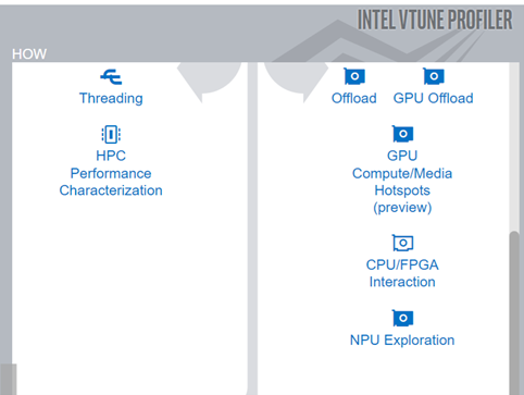
For NPU Analysis, you need to choose the NPU Exploration from the list of Analysis Options.

There are two data collection modes, with different purposes

• Time-based: collects system-wide metrics
  • Use for larger workloads
  • Less overhead
• Query-based: collects metrics for each instance of a Level Zero instance
  • Use for smaller workloads
  • Higher overhead

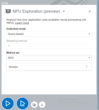
Currently, the only Metric Set Supported is NOC (Network-on-Chip) fabric. The NPU goes through this fabric to read/write data from/to DDR memory. The sampling Interval can also be set based on your workload and required profiling granularity. Other detailed options can be set from the “How pane” for more fine-grained control.

You can also run this analysis from the command line. Here is a sample command line format for the NPU exploration analysis.

Common format:

vtune -collect npu [-knob <knob_name=knob_option>] -- <target> [target_options]

In this example, we will run a mobilenet-v2 model on NPU and profile the application with VTune’s  NPU exploration analysis.

Original Sample Code

mobilnet_unoptimized.py:

import re
import subprocess
from pathlib import Path
from typing import List

import numpy as np
import openvino as ov
import torch
from fastdownload import FastDownload
from rich.progress import track
from sklearn.metrics import accuracy_score
from torchvision import datasets
from torchvision import transforms

import nncf

ROOT = Path(__file__).parent.resolve()
DATASET_PATH = Path().home() / ".cache" / "nncf" / "datasets"
MODEL_PATH = Path().home() / ".cache" / "nncf" / "models"
MODEL_URL = "https://huggingface.co/alexsu52/mobilenet_v2_imagenette/resolve/main/openvino_model.tgz"
DATASET_URL = "https://s3.amazonaws.com/fast-ai-imageclas/imagenette2-320.tgz"
DATASET_CLASSES = 10


def download(url: str, path: Path) -> Path:
    downloader = FastDownload(base=path.resolve(), archive="downloaded", data="extracted")
    return downloader.get(url)


def validate(model: ov.Model, val_loader: torch.utils.data.DataLoader) -> float:
    predictions = []
    references = []

    compiled_model = ov.compile_model(model, device_name="NPU")
    output = compiled_model.outputs[0]

    for images, target in track(val_loader, description="Validating"):
        pred = compiled_model(images)[output]
        predictions.append(np.argmax(pred, axis=1))
        references.append(target)

    predictions = np.concatenate(predictions, axis=0)
    references = np.concatenate(references, axis=0)
    return accuracy_score(predictions, references)


def run_benchmark(model_path: Path, shape: List[int]) -> float:
    cmd = ["benchmark_app", "-m", model_path.as_posix(), "-d", "GPU", "-api", "async", "-niter", "50000", "-shape", str(shape)]
    cmd_output = subprocess.check_output(cmd, text=True)  # nosec
    print(*cmd_output.splitlines()[-8:], sep="\n")
    match = re.search(r"Throughput\: (.+?) FPS", cmd_output)
    return float(match.group(1))


def get_model_size(ir_path: Path, m_type: str = "Mb") -> float:
    xml_size = ir_path.stat().st_size
    bin_size = ir_path.with_suffix(".bin").stat().st_size
    for t in ["bytes", "Kb", "Mb"]:
        if m_type == t:
            break
        xml_size /= 1024
        bin_size /= 1024
    model_size = xml_size + bin_size
    print(f"Model graph (xml):   {xml_size:.3f} Mb")
    print(f"Model weights (bin): {bin_size:.3f} Mb")
    print(f"Model size:          {model_size:.3f} Mb")
    return model_size


###############################################################################
# Create an OpenVINO model and dataset

dataset_path = download(DATASET_URL, DATASET_PATH)

normalize = transforms.Normalize(mean=[0.485, 0.456, 0.406], std=[0.229, 0.224, 0.225])
val_dataset = datasets.ImageFolder(
    root=dataset_path / "val",
    transform=transforms.Compose(
        [
            transforms.Resize(256),
            transforms.CenterCrop(224),
            transforms.ToTensor(),
            normalize,
        ]
    ),
)
val_data_loader = torch.utils.data.DataLoader(val_dataset, batch_size=1, shuffle=False)

path_to_model = download(MODEL_URL, MODEL_PATH)
ov_model = ov.Core().read_model(path_to_model / "mobilenet_v2_fp32.xml")

###############################################################################
# Quantize an OpenVINO model
#
# The transformation function transforms a data item into model input data.
#
# To validate the transform function use the following code:
# >> for data_item in val_loader:
# >>    model(transform_fn(data_item))


def transform_fn(data_item):
    images, _ = data_item
    return images

calibration_dataset = nncf.Dataset(val_data_loader, transform_fn)
ov_quantized_model = nncf.quantize(ov_model, calibration_dataset)

###############################################################################
# Benchmark performance, calculate compression rate and validate accuracy

fp32_ir_path = ROOT / "mobilenet_v2_fp32.xml"
ov.save_model(ov_model, fp32_ir_path, compress_to_fp16=False)
print(f"[1/7] Save FP32 model: {fp32_ir_path}")
fp32_model_size = get_model_size(fp32_ir_path)

print("[3/7] Benchmark FP32 model:")
fp32_fps = run_benchmark(fp32_ir_path, shape=[1, 3, 224, 224])

Sample Command Line:

vtune -c npu --  python mobilnet_unoptimized.py

3. Interpret the Results

You can see the NPU exploration results by launching the VTune Profiler GUI and opening the .vtune file.

Top Task Overview

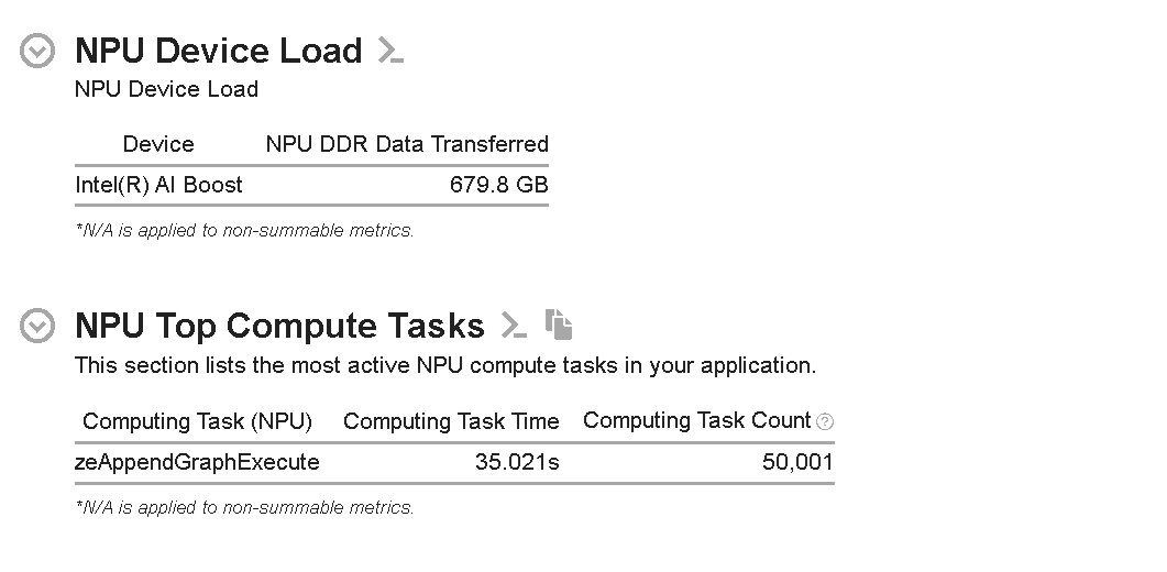
Figure 1: Summary View of NPU Exploration Analysis

The NPU Device Load section shows the data transferred from DDR SDRAM to NPU through NOC. As can be seen from Figure 1, the amount of data transferred is 679.8 GB.

Also, a “NPU Top Compute Tasks” section lists the top computing tasks executing on the NPU side. In this example,  zeAppendGraphExecute appends a graph execution command to the command list. These API calls take ~35s to execute any number of tasks, and the count is 50,001. In this context, a graph represents a sequence of operations that can be executed on the NPU.

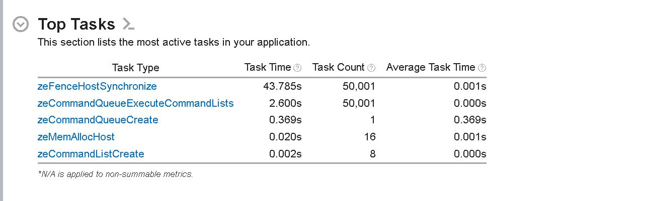
Figure 2: List of Top Tasks on the Host Side

The ’Top Tasks’ section lists the most active tasks taking place on the host side execution of the application. This section helps identify which functions or code regions consume the most CPU time. The most time-consuming host tasks are zeFenceHostSynchronize API calls that take ~54s. These calls ensure the host waits until the fence is signaled or a specified timeout period expires. This list shows the total time taken by each task, the total task count, and the average time for each task.

A Deeper Look

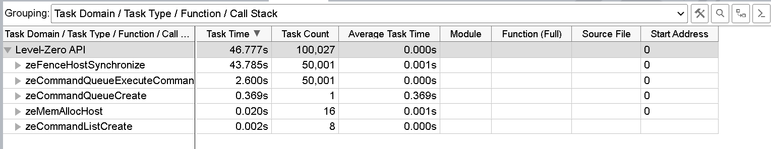
Figure 3: Bottom-Up View of NPU and Host Tasks

The next step is to investigate each task more deeply. For that, you need to go to the Bottom-Up view. In this view, you can see the execution timeline and a bottom-up view of the functions and tasks based on specified Grouping.

The recommended grouping is Task Type/Function/Call Stack for understating the NPU and Host tasks.

Figure 4 (timeline view) shows the list of threads running on the CPU and NPU. You can also see the corresponding NPU Utilization and NPU Bandwidth throughout the timeline. Here, we select the region where the NPU was active and can see the duration for inference is ~54s.

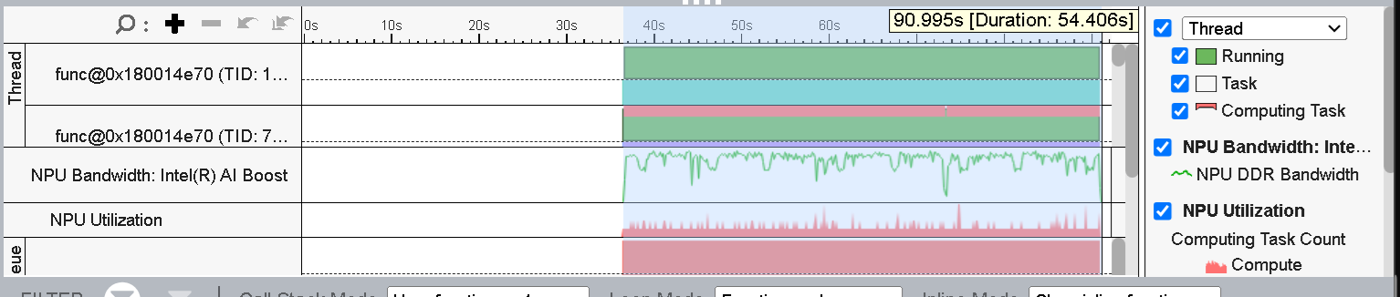
Figure 4: Timeline view of the Application Execution

The rest of the execution time (first 35s) is spent on other CPU tasks (Statistical Collection, Fast Bias Correction). You can see more details on CPU activity by expanding the ‘Thread’ section.

As Figure 5 shows, CPU tasks like Memory Allocation and Queue Creation occur right before the inference starts.

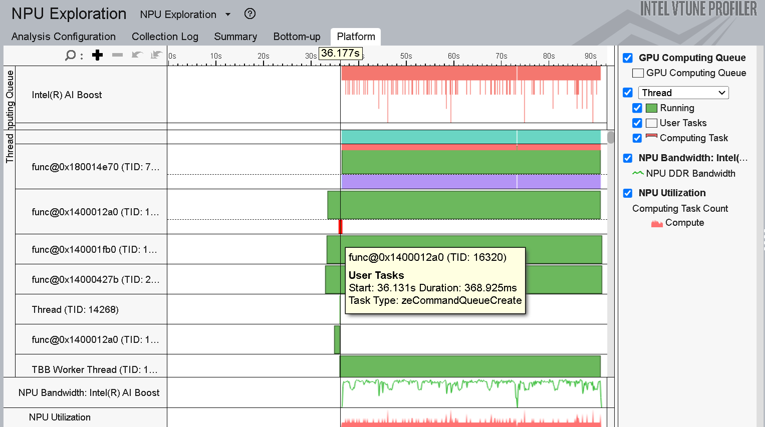
Figure 5: Expanded view of the Thread section of Bottom-up viewpoint

If you see a dip in the NPU Utilization or NPU Bandwidth you can zoom into that time slice and see the corresponding CPU and NPU tasks to understand the API or the tasks causing the performance loss.

Whenever there is a dip in NPU utilization or NPU Bandwidth, a host-side task occurs (marked in purple). To better understand, you can expand the corresponding thread and hover over the task to see the details.

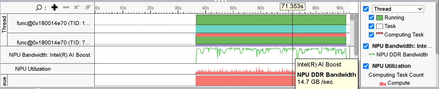
Figure 6: NPU DDR Bandwidth

From the timeline view, we can also see the NPU DDR Bandwidth utilization throughout the execution time.  The Figure 6 shows that the peak NPU DDR Bandwidth is ~14 GB/s.

Typical NPU Utilization Bottlenecks

Bottlenecks Observed Using Intel VTune Profiler:

1. High DDR to NPU data transfer adding to the data transfer overhead
2. High Pressure on NPU Memory
3. Significant time spent on host-side synchronization
4. Dip in the NPU Utilization and NPU Bandwidth Utilization

Recommendation

When possible, use lower-precision data to reduce the amount of data transfer and pressure on the memory subsystem. Lower-precision data reduces latency in host-device communication, alleviating the synchronization overhead.

4. Optimize the Workload Based on the Results

In this step, we apply an optimization technique based on the bottlenecks we observed using Intel VTune Profiler. We will quantize the model using the Neural Network Compression Framework (NNCF) Post-Training Quantization algorithm. The goal of quantization is to reduce the pressure on the memory subsystem per the recommendation above.

Changes Made for Code Optimization:

• Quantized the FP32 model using the nncf.quantize function with a calibration dataset.
• Saved the quantized  model after quantization.
• Benchmarked the quantized model for NPU device.

import re
import subprocess
from pathlib import Path
from typing import List

import numpy as np
import openvino as ov
import torch
from fastdownload import FastDownload
from rich.progress import track
from sklearn.metrics import accuracy_score
from torchvision import datasets
from torchvision import transforms

import nncf

ROOT = Path(__file__).parent.resolve()
DATASET_PATH = Path().home() / ".cache" / "nncf" / "datasets"
MODEL_PATH = Path().home() / ".cache" / "nncf" / "models"
MODEL_URL = "https://huggingface.co/alexsu52/mobilenet_v2_imagenette/resolve/main/openvino_model.tgz"
DATASET_URL = "https://s3.amazonaws.com/fast-ai-imageclas/imagenette2-320.tgz"
DATASET_CLASSES = 10


def download(url: str, path: Path) -> Path:
    downloader = FastDownload(base=path.resolve(), archive="downloaded", data="extracted")
    return downloader.get(url)


def validate(model: ov.Model, val_loader: torch.utils.data.DataLoader) -> float:
    predictions = []
    references = []

    compiled_model = ov.compile_model(model, device_name="NPU")
    output = compiled_model.outputs[0]

    for images, target in track(val_loader, description="Validating"):
        pred = compiled_model(images)[output]
        predictions.append(np.argmax(pred, axis=1))
        references.append(target)

    predictions = np.concatenate(predictions, axis=0)
    references = np.concatenate(references, axis=0)
    return accuracy_score(predictions, references)


def run_benchmark(model_path: Path, shape: List[int]) -> float:
    cmd = ["benchmark_app", "-m", model_path.as_posix(), "-d", "GPU", "-api", "async", "-niter", "50000", "-shape", str(shape)]
    cmd_output = subprocess.check_output(cmd, text=True)  # nosec
    print(*cmd_output.splitlines()[-8:], sep="\n")
    match = re.search(r"Throughput\: (.+?) FPS", cmd_output)
    return float(match.group(1))


def get_model_size(ir_path: Path, m_type: str = "Mb") -> float:
    xml_size = ir_path.stat().st_size
    bin_size = ir_path.with_suffix(".bin").stat().st_size
    for t in ["bytes", "Kb", "Mb"]:
        if m_type == t:
            break
        xml_size /= 1024
        bin_size /= 1024
    model_size = xml_size + bin_size
    print(f"Model graph (xml):   {xml_size:.3f} Mb")
    print(f"Model weights (bin): {bin_size:.3f} Mb")
    print(f"Model size:          {model_size:.3f} Mb")
    return model_size


###############################################################################
# Create an OpenVINO model and dataset

dataset_path = download(DATASET_URL, DATASET_PATH)

normalize = transforms.Normalize(mean=[0.485, 0.456, 0.406], std=[0.229, 0.224, 0.225])
val_dataset = datasets.ImageFolder(
    root=dataset_path / "val",
    transform=transforms.Compose(
        [
            transforms.Resize(256),
            transforms.CenterCrop(224),
            transforms.ToTensor(),
            normalize,
        ]
    ),
)
val_data_loader = torch.utils.data.DataLoader(val_dataset, batch_size=1, shuffle=False)

path_to_model = download(MODEL_URL, MODEL_PATH)
ov_model = ov.Core().read_model(path_to_model / "mobilenet_v2_fp32.xml")

def transform_fn(data_item):
    images, _ = data_item
    return images


calibration_dataset = nncf.Dataset(val_data_loader, transform_fn)
ov_quantized_model = nncf.quantize(ov_model, calibration_dataset)

###############################################################################
# Benchmark performance, calculate compression rate and validate accuracy

int8_ir_path = ROOT / "mobilenet_v2_int8.xml"
ov.save_model(ov_quantized_model, int8_ir_path)
print(f"[2/7] Save INT8 model: {int8_ir_path}")
int8_model_size = get_model_size(int8_ir_path)

print("[4/7] Benchmark INT8 model:")
int8_fps = run_benchmark(int8_ir_path, shape=[1, 3, 224, 224])

After applying the optimization, we will inspect the following metrics using VTune Profiler:

1. Understanding the change in the DDR to NPU Data transferred.
2. Observing the inference time from the VTune’s timeline view.
3. Checking the peak NPU memory bandwidth.

Observed Execution Speedup

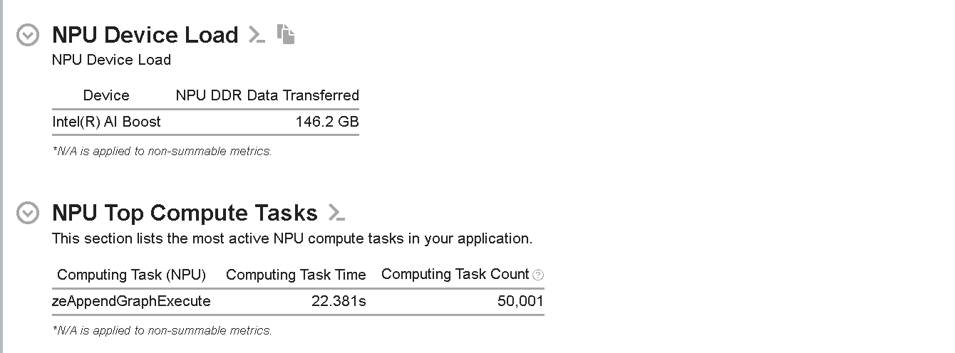
Figure 7: NPU Device Load and NPU Top Compute Tasks for Quantized Model

As can be seen from Figure 7, the NPU Device Load has dropped from ~680 GB to ~146 GB, which is almost a 78.5% improvement in the NPU DDR Data Transferred. Improving the Data Transfer Overhead should accelerate the inference time on NPU.

Also, the NPU Top Compute Tasks section shows that the top time-consuming task, zeAppendGraphExecute, now takes only ~22s, which is a 37.14% improvement.

Figure 8: Top Tasks on the Host side after quantization

We can also see significant differences in the Top tasks on the host side. For example, the zeFenceHostSynchronize and zeCommandQueueExecuteCOmmandLists now take much less time compared to the unquantized implementation of the model.

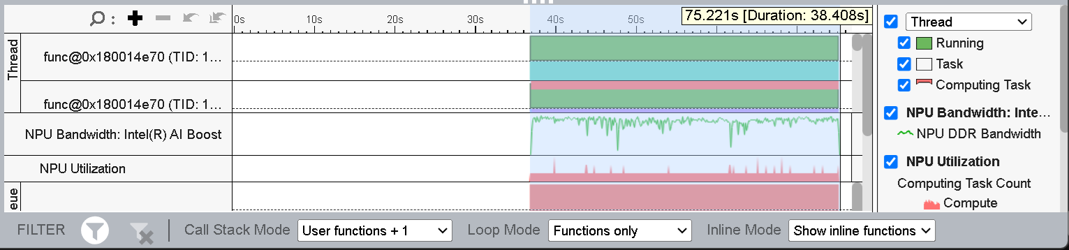
Figure 9: Inference Time of the quantized model (Timeline View)

As seen in Figure 9, the duration of the inference is now ~38s, which has sped up significantly (30%) from the previous implementation. You should be able to see the inference time by selecting the timeline while the NPU was active.

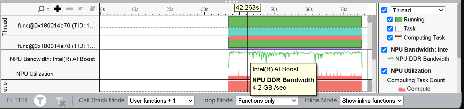
Figure 10: NPU Bandwidth of the quantized Model

As can be seen from Figure 10, the peak NPU DDR Bandwidth has dropped from ~14 GB/s to ~4 GB/s. That will also reduce the NPU Memory activity and DDR to NPU data transfer, which significantly improves the overall inference performance.

Test it Yourself

To walk through these steps yourself and apply them to your own application, you can simply do the following:

• Set up your own environment as described at the beginning of this article.
• Run any examples provided here, or use your own development project.
• Profile the application using Intel VTune Profiler to detect and then fix any bottlenecks.

Get the Software

You can install Intel VTune Profiler as a part of the Intel® oneAPI Base Toolkit or download its stand-alone version for free! 

Streamline your software setup with our toolkit selector to install full kits or new, right-sized sub-bundles containing only the needed components for specific use cases! Save time, reduce hassle, and get the perfect tools for your project with Intel® C++ Essentials, Intel® Fortan Essentials, and Intel® Deep Learning Essentials.