In the domain of computer vision, image transformation techniques serve as critical preprocessing tools that ensure consistency, alignment, and geometric normalization across datasets.
The Intel® Integrated Performance Primitives (Intel® IPP) enables developers to use ippiWarpAffine and ippiWarpPerspective functions to implement affine and perspective transformations in C/C++ code. Similarly, the OpenCV library provides C++ APIs and Python interfaces through cv2.warpAffine and cv2.warpPerspective. These functions apply affine and perspective (projective) transformations respectively and serve as foundational building blocks in a wide variety of applications—ranging from document OCR to security cameras and medical devices. Intel® IPP provides hardware-accelerated implementations of these functions optimized for Intel® SSE4/Intel® AVX2 and Intel® AVX-512 capable processors. At the time of writing, this article uses Intel® IPP 2026.0.0 and OpenCV 4.13 as the reference versions.
Typical use cases for warp transformations include the following:
-
Document Scanning and Recognition: Correcting skewed photos of documents is essential to prepare scans using phones or for accurate text recognition (Optical Character Recognition, or OCR). OCR pipelines require text to be aligned horizontally, as images scanned or photographed at a slight angle can lead to significant recognition errors if left uncorrected. Warp perspective transformation allows preprocessing of entire image datasets before feeding them into OCR systems such as Tesseract.
-
Panorama Stitching: When creating panoramic images, multiple overlapping photos must be aligned and blended seamlessly. Warp transformations enable the geometric alignment necessary to merge these images into a single cohesive panorama.
-
Face Alignment: Facial recognition systems often require aligned input for optimal accuracy. By detecting facial landmarks and applying warp transformations to normalize the pose, developers can significantly increase model accuracy and consistency across different input images.
-
Medical Image Registration: Slices from MRI (magnetic resonance imaging) or CT (computed tomography) scans may be slightly misaligned due to patient movement or equipment variations. Warp transformations help adjust these slices for accurate 3D reconstructions or comparative analysis over time.
-
Autonomous Driving Vision: Processing road signs and lane markings involves traffic sign rectification and lane detection (generating Bird's-Eye View). Since the moving camera is not directly perpendicular to the sign or road plane, road signs, although planar, appear as trapezoids rather than rectangles due to perspective distortion. Perspective warping (using 3x3 matrices) can rectify this, transforming a slanted sign into a frontal, rectangular view, making it easier for Deep Neural Networks (DNNs) like SignNet to classify them. Since the camera is moving fast, the performance is critical for that task.
The article covers the basics of warp operations in the Intel® IPP and OpenCV libraries. The document scanning and alignment case in a computer vision batch-processing workload will be covered in detail in the next sections, with an example of an efficient implementation in Python code. In conclusion, the performance measurements will be provided and analyzed, and it will be explained how the code can be accelerated on Intel® Xeon® 6 Processors with P-cores in the most efficient way.
Warp transformations
Warp transformations can be classified into two main types: warp affine and warp perspective.
An affine transformation is a geometric mapping that preserves line and plane parallelism and ratios of distances between points using linear transformations. The transformation consists of several basic geometric operations:
- Translation: Shifting the image horizontally or vertically
- Rotation: Rotating the image around a point
- Scaling: Enlarging or shrinking the image
- Shearing: Skewing the image along an axis
2D warp affine APIs use a 2×3 matrix to apply these transformations. The warp affine transformation can be mathematically represented as:
$$\begin{bmatrix} x' \\ y' \end{bmatrix} = \begin{bmatrix} h_{00} & h_{01} & h_{02} \\ h_{10} & h_{11} & h_{12} \end{bmatrix} \begin{bmatrix} x \\ y \end{bmatrix}$$
The warp affine matrix can be generated using helper functions provided by the library. For example, OpenCV provides the following Python functions to generate rotation or custom affine transformation matrices:
cv2.getRotationMatrix2D(center, angle, scale)
cv2.getAffineTransform(src_pts, dst_pts)
Here, src_pts and dst_pts are arrays of three corresponding points that define the transformation. That means that as a result of transformation the source points are mapped to the destination points one by one in the same order.
Unlike warp affine (which uses a 2×3 matrix for rotation, scale, and shear), warp perspective uses a 3×3 homography matrix to perform a full projective transformation. This accounts for changes in perspective, such as tilting or keystoning.
The warp perspective transformation can be represented as:
$$\begin{bmatrix} x' \\ y' \\ w \end{bmatrix} = \begin{bmatrix} h_{00} & h_{01} & h_{02} \\ h_{10} & h_{11} & h_{12} \\ h_{20} & h_{21} & h_{22} \end{bmatrix}\begin{bmatrix} x \\ y \\ 1 \end{bmatrix}$$
The warp perspective matrix can be generated using helper functions provided by image processing libraries. For example, OpenCV provides the following Python function to generate a perspective transformation matrix:
H = cv2.getPerspectiveTransform(src_pts, dst_pts)
The points do not technically have to be ordered in clockwise or counter-clockwise direction, but they must follow a strict ordered sequence — commonly top-left, top-right, bottom-right, and bottom-left. Alternatively, if dealing with an arbitrary number of points or in the case of potential outliers (panorama stitching case), a universal and robust function should be used to determine the transformation matrix:
H, _ = cv2.findHomography(src_pts, dst_pts)
Here, src_pts and dst_pts are arrays of four corresponding points that define the perspective transformation. Unlike affine transformations, perspective transformations require four points because they can represent more complex geometric distortions.
That is the basic idea of warp transformation, with Python code snippets using the OpenCV library to compute transformation matrices based on points. To use OpenCV, Python code is required; for the Intel® IPP library, C code must be written, which requires additional effort and is covered in the next sections.
How to use warp transformations in Intel® IPP
The Intel® IPP library provides the ippiWarpAffine family of functions to implement affine transformations using pre-calculated affine coefficients based on rotation parameters (angle, x-shift, and y-shift). To apply the transform, you need to define the affine transform coefficients, which can be done either manually or by using helper functions. To obtain affine coefficients for specified rotation parameters, you can use the ippiGetRotateTransform function. This function computes the affine coefficients for a transform that rotates an image by a specified angle around the origin (0, 0) and shifts the image by specified x and y values.
// compute affine transform matrix to perform rotation around (0,0) by angle
double   coeffs[2][3] = {0};
status = ippiGetRotateTransform(angle, 0, 0, coeffs);
For a generic affine transform, the ippiGetAffineTransform function should be used, providing the roi (region of interest, which is rectilinear and defined by 4 points) and quad, which is an affine-transformed representation of the roi rectangle.
// compute affine transform matrix for a generic affine transform
double   coeffs[2][3] = {0};
status = ippiGetAffineTransform(roi, quad, coeffs);
Before calling the warp affine processing function, the following steps are required:
- Compute the specification structure size and allocate memory for it for affine warping with the specified interpolation method using the
ippiWarpAffineGetSize/ippiWarpPerspectiveGetSizefunction. - Initialize the specification structure using functions based on interpolation. For linear interpolation, which is generally used by default to balance computing performance and image quality, the
ippiWarpAffineLinearInit/ippiWarpPerspectiveLinearInitfunction shall be used. - Compute the temporary work buffer size required for warping using
ippiWarpGetBufferSize, then allocate the buffer and pass its pointer to the processing function.
The code example below demonstrates how to perform these 3 steps for warp perspective transformation using Intel® IPP if we wanted to align the page by deskewing using single-channel unsigned int image data (Ipp8u). roi and roiSize in this case are the image size (width, height), since no special computing of reduced roi is performed. The transformation direction is ippWarpBackward:
    int srcStep = width * sizeof(Ipp8u);
    int dstStep = srcStep;
    int bufSize = 0, specSize = 0;
    IppiPoint roiOffset = {0, 0};
    IppiSize roiSize = {width, height};
    IppiRect roi = {0, 0, width, height};
    double borderValue = 128.0;

    status = ippiGetPerspectiveTransform(roi, quad, H);

    // 1. Compute the specification structure size
    status = ippiWarpPerspectiveGetSize(
        roiSize, roi, roiSize, ipp8u, H,
        ippLinear, ippWarpBackward, ippBorderConst,
        specSize, bufSize);

    // Allocate memory for specification structure
    IppiWarpSpec* pSpec = (IppiWarpSpec*)ippMalloc_L(*specSize);
    if (pSpec == NULL) {
        return ippStsMemAllocErr;
    }

    // 2. Initialize the specification structure
    status = ippiWarpPerspectiveLinearInit(
        roiSize, roi, roiSize, ipp8u, H,
        ippWarpBackward, 1, ippBorderConst, &borderValue, 0, pSpec);

    // 3. Compute the temporary work buffer size
    status = ippiWarpGetBufferSize(pSpec, roiSize, bufSize);
The code example below demonstrates how to perform image warp perspective transformation after the sizes of the structure and buffer are computed. Single-channel, unsigned 8-bit integer images are used. Warp perspective is performed with linear interpolation. Status checks should be performed in production code; here they are skipped for simplicity and to reduce code snippet size.
    int srcStep = width * sizeof(Ipp8u);
    int dstStep = srcStep;
    int bufSize = 0, specSize = 0;
    IppiPoint roiOffset = {0, 0};
    IppiSize roiSize = {width, height};
    IppiRect roi = {0, 0, width, height};
    double borderValue = 128.0;

    IppiWarpSpec* pSpec = (IppiWarpSpec*)ippMalloc_L(specSize);
    Ipp8u* pBuf = (Ipp8u*)ippMalloc_L(bufSize);

    // Process a batch of images of size N
    for (int i = 0; i < N; i++) {

        // Get pointers to the frame points for this image (8 floats = 4 points x 2 coords) and convert to double
        float *srcPts = (float*)(&srcPtsArray[i * 8]);
        const double quad[4][2] = {
            { srcPts[0], srcPts[1] },
            { srcPts[2], srcPts[3] },
            { srcPts[4], srcPts[5] },
            { srcPts[6], srcPts[7] }
        };
        Ipp64f H[3][3] = {{1,0,0},{0,1,0},{0,0,1}};
        status = ippiGetPerspectiveTransform(roi, quad, H);

        // Initialize warp structure for this transform
        status = ippiWarpPerspectiveLinearInit(
            roiSize, roi, roiSize, dataType, H,
            ippWarpBackward, 1, ippBorderConst, &borderValue, 0, pSpec);

        // Perform the warp transformation
        status = ippiWarpPerspectiveLinear_8u_C1R(
            pSrcArray, srcStep,
            pDstArray, dstStep,
            roiOffset, roiSize,
            pSpec, pBuf
        );
    }

    // Free buffers
    ippFree(pBuf);
    ippFree(pSpec);
How to use warp transformations in OpenCV
Implementing warp affine and perspective transformations in OpenCV is straightforward with Python. The following helper functions demonstrate how to apply these transformations to an image:
def affine_transform(image, quad):
    h, w = image.shape
    dst = np.float32([[0, 0], [w - 1, 0], [w - 1, h - 1]])
    M = cv2.getAffineTransform(quad[:3], dst)
    return cv2.warpAffine(image, M, (w, h))

def perspective_transform(image, quad):
    h, w = image.shape
    dst = np.float32([[0, 0], [w - 1, 0], [w - 1, h - 1], [0, h - 1]])
    H = cv2.getPerspectiveTransform(quad, dst)
    return cv2.warpPerspective(image, H, (w, h))
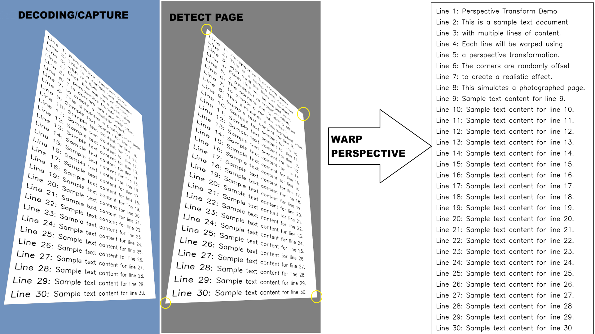
Let's consider a batch processing example that performs warp transformations on multiple images. This is a typical scenario for page alignment, where pages need to be extracted and straightened from photos or video frames.
OpenCV uses an internal threading implementation for parallelization, so we'll introduce a num_threads parameter to control the number of threads. We'll also add an affine flag to indicate whether to use warp affine (when True) or warp perspective (when False).
For this example, we focus solely on the warp transformations themselves. The corner points defining the warp are assumed to be precomputed; this can be achieved using OpenCV's findContours functionality or other contour detection methods.
def batch_warp_transform(warped_images, dewarped_images, warp_points, affine=False, num_threads=1):
    cv2.setNumThreads(num_threads)
    if(affine):
        for i, (image, point) in enumerate(zip(warped_images, warp_points)):
            dewarped_images[i] = affine_transform(image, point)
    else:
        for i, (image, point) in enumerate(zip(warped_images, warp_points)):
            dewarped_images[i] = perspective_transform(image, point)
Achieving the same result using Intel® IPP directly requires C programming, which leads to significantly more code. This approach will be partially covered in later sections, and the full example can be found at Intel Samples.
Once you have a dataset of warped images or captured video frames from a camera source, you can use simple Python code like the examples above to measure and compare performance between different implementations.
The performance estimations are based on our internal testing using a Python sample that performs a pipeline of decoding, contour detection, and warp perspective. In the experimental pipeline with decoded image sources, the goal is to achieve 30 frames per second (FPS) throughput. The point of interest is to estimate which computational resources might be needed to achieve the 30 FPS processing throughput. Decoding is a hardware operation with almost no overhead on the CPU, and contour detection is quite a heavy operation—warp perspective takes about 10% of the entire pipeline. If we consider other functions are not the optimization target and operate at maximum speed, then to achieve 30 FPS, the warp perspective transformation must achieve 300 FPS.
A later section estimates the performance and demonstrates for which resolutions this is possible on Intel® Xeon® 6 CPUs.
Comparing warp code performance of implementations based on Intel® IPP and OpenCV
Performance testing methodology and configuration
For this performance comparison, we tested Intel® IPP 2026.0.0 and OpenCV v4.13. Intel® IPP includes optimized warp affine and perspective implementations for both AVX2 and AVX-512 hardware. Performance testing was conducted on an Intel® Xeon® 6 because Intel® IPP 2026.0 includes specific optimizations for warp perspective operations on the AVX-512 instruction set. The test CPU features performance cores, and in the default configuration, each NUMA node consists of 32 physical cores. All workloads were executed within a single NUMA node to ensure consistent memory access patterns. All benchmarks are performed on a single node with 2x Intel® Xeon® 6972P processor on AvenueCity platform with 1536 GB (24 slots/ 64GB/ 8800) total DDR5 memory, HT on, Turbo on, Ubuntu 24.04 LTS, 6.8.0-90-generic kernel with Python 3.12.4. A single CPU has 96 cores which are clustered into 3 NUMA nodes with 32 cores each. We considered a single NUMA node case in this paper, since it is sufficient for most cases and was not affected by NUMA impact. For tuning on multiple NUMA nodes you need to apply advanced techniques on memory and thread scheduling, according to the Performance tuning guide for Intel® Xeon® 6.
The benchmark runs warp perspective on 8-bit unsigned integer data to align the warped page for images across various resolutions in the table below.
| Format | Resolution | Description |
|---|---|---|
| FHD | 1920 × 1080 | Full HD video |
| 2K | 2560 × 1440 | QHD/2K video |
| 4K | 3840 × 2160 | Ultra HD video |
| 8K | 7680 × 4320 | 8K Ultra HD video |
| 12MP | 3024 × 4032 | Smartphone camera |
| 50MP | 6144 × 8192 | Professional camera |
| 200MP | 12320 × 16224 | High-resolution sensor |
The benchmark performs multiple runs and computes the throughput in frames per second (FPS) for the computational part and selects the median value to remove all potential outliers. The latest version of the Intel® IPP library (2026.0.0) has improved optimizations for Intel® Xeon® 6 CPU warp functionality by implementing optimizations with the AVX-512 instruction set, which makes execution several times faster compared to the OpenCV library, including the use case considered in this paper, which is demonstrated in the following sections.
Intel® IPP integration in OpenCV
OpenCV 4.13 includes Intel® IPP integration to accelerate computer vision operations on Intel CPUs. However, the warp perspective functionality covered in this article differs in precision characteristics because Intel® IPP implements the optimized algorithm differently than OpenCV's native implementation. As a result, the Intel® IPP-accelerated warp perspective is not enabled by default in OpenCV builds.
If precision alignment with native OpenCV behavior is not critical for your application, you can enable Intel® IPP-accelerated warp functions by setting a specific CMake build flag:
cmake -DWITH_IPP=ON -DWITH_IPP_CALLS_ENFORCED=ON ..
make
make install
For the use cases considered in this article, which do not involve extreme transformations, approximately 10-15% of pixels showed differences between the Intel® IPP and native OpenCV implementations. This level of difference is generally acceptable for many practical applications.
In the upcoming OpenCV 5.x release, it is expected that precision control through an algorithm hint parameter will enable more Intel® IPP functions to be used in the implementation, including 8-bit unsigned integer (8U) operations, which are very common in standard image processing workflows.
The enforced integration almost aligns the OpenCV and Intel® IPP performance; however, the pure Intel® IPP implementation is still slightly faster (the data is collected on the hardware configuration described above).
Since Intel® IPP functions are single-threaded by design, we first measured the single-threaded warp perspective performance on the hardware described above. For the multithreaded performance measures, additional considerations were applied and are described in the paper along with the achieved results.
Ways to improve warp code performance
OpenCV operations with Intel® IPP integration work in a straightforward manner, performing the same set of operations for both multithreaded and single-threaded execution. However, since most Intel® IPP functions, including warp operations, require memory allocation, the repeated allocation and deallocation of memory introduces significant overhead.
The typical sequence used in each OpenCV threaded call involves the following steps:
- Detect memory size
- Allocate memory
- Compute warp transformation matrix and initialize warp
- Compute warp
- Deallocate memory
Notice that only the compute-related steps (3 and 4) are unique for each image in the batch and the memory operations are redundant overhead. Using Intel® IPP directly provides a more flexible solution that can optimize threading and memory management for batch processing. As with the OpenCV implementation, native code written in C handles threading and memory allocations. To provide a convenient Python interface, a binding library such as Cython should be used.
When combining Intel® IPP with Cython for optimal memory efficiency and computational performance, the implementation should follow these key principles:
- Zero-copy memory access and contiguous memory layout between Python and C.
- Thread-local buffer allocation for parallel processing, reducing allocations and deallocations by reusing the buffers across the batch subset processed by a specific thread.
- Parallelization with proper thread safety.
To build such a solution for Python, we implement a three-layer architecture:
- Python Layer: Works with NumPy arrays for seamless integration with Python code
- Cython Layer: Handles validation and bridges Python to C function calls
- C Layer: Implements the core functionality using Intel® IPP with OpenMP for threading
Python API
We keep the Python API consistent with the earlier OpenCV examples, making it easy to swap implementations:
# Same interface as the OpenCV version
batch_warp_transform(src_images, dst_images, src_points, affine=False, num_threads=1)
Cython bindings
With a contiguous memory layout, PyArray_DATA is used to obtain direct access to NumPy array data in C code for all data arrays (source images, destination images, and warp points). Cython also provides validation to ensure contiguous memory layout through the flags['C_CONTIGUOUS'] attribute:
# batch_warp.pyx
import numpy as np
cimport numpy as cnp

def batch_warp_transform(src_images, dst_images, src_points, ...):
    # Validate contiguity FIRST
    if not src_images.flags['C_CONTIGUOUS']:
        raise ValueError("src_images must be C-contiguous")
    ...

    # Get direct pointer to NumPy array data - NO COPY
    cdef void* pSrcData = <void*>cnp.PyArray_DATA(src_images)
    cdef void* pDstData = <void*>cnp.PyArray_DATA(dst_images)
    cdef float* pSrcPtsArray = <float*>cnp.PyArray_DATA(src_points)

    # Pass pointers directly to C function
    status = BatchWarpPerspective(
        pSrcData, pDstData, pSrcPtsArray,
        N, width, height, num_threads, isFloat
    )
C code implementation
Image transformation requires temporary buffers for Intel® IPP's internal calculations. A key optimization is that these buffers can be reused across multiple images in a batch, since the buffer size is determined by the destination dimensions, which are uniform across the batch.
The strategy is for each thread to allocate its own memory buffers once, then reuse them for all images that thread processes. In OpenMP, this is implemented by placing memory allocation inside the #pragma omp parallel region but before the #pragma omp for loop, allowing buffers to be shared across loop iterations within each thread:
// batch_warp_core.c

// Calculate buffer sizes once for uniform batch
int bufSize = 0, specSize = 0;
GetPerspectiveBufferSizes(
    roiSize, roi, dataType, srcPtsArray,
    borderValue, &specSize, &bufSize);

// Parallel region with thread-local storage
#pragma omp parallel num_threads(numThreads) shared(finalStatus)
{
    // Each thread allocates its own buffers ONCE
    IppiWarpSpec* pSpec = (IppiWarpSpec*)ippMalloc_L(specSize);
    Ipp8u* pBuf = (Ipp8u*)ippMalloc_L(bufSize);

    if (pSpec == NULL || pBuf == NULL) {
        #pragma omp critical
        finalStatus = ippStsMemAllocErr;
    }

    // Process multiple images with same buffers
    #pragma omp for
    for (int i = 0; i < N; i++) {
        // Each thread processes different images
        // Reuses pSpec and pBuf for every image
        size_t imageOffset = (size_t)i * width * height;

        // Compute transformation for this image
        ippiGetPerspectiveTransform(roi, quad, H_local);
        ippiWarpPerspectiveLinearInit(..., pSpec);

        // Apply transformation
        ippiWarpPerspectiveLinear_8u_C1R(
            ((Ipp8u*)pSrcArray) + imageOffset, srcStep,
            ((Ipp8u*)pDstArray) + imageOffset, dstStep,
            roiOffset, roiSize,
            pSpec, pBuf  // Thread-local buffers
        );
    }

    // Free thread-local buffers ONCE per thread
    ippFree(pBuf);
    ippFree(pSpec);
}
Synchronization is only required for the shared error status (finalStatus variable), which is protected using #pragma omp critical. This minimal synchronization ensures thread safety without introducing significant overhead.
The memory allocation optimization provides significant improvements. For processing 192 images with 8 threads:
- without optimization: 192 allocations × 2 buffers = 384 malloc/free calls
- with thread-local buffers: 8 threads × 2 buffers = 16 malloc/free calls
This represents a significant reduction in memory allocation overhead, which significantly improves scalability.
Memory layout
The batch of images is stored as a single contiguous 3D NumPy array:
# Python side: Create contiguous batch
src_images = np.zeros((N, height, width), dtype=np.uint8)  # C-contiguous by default
With this layout, each image immediately follows the previous one in memory, enabling efficient pointer arithmetic in the C code to access individual images within the batch.
Performance results
The batch processing implementation with Intel® IPP calls outperforms OpenCV with a stable performance advantage on a specific number of threads on Intel® Xeon® 6:
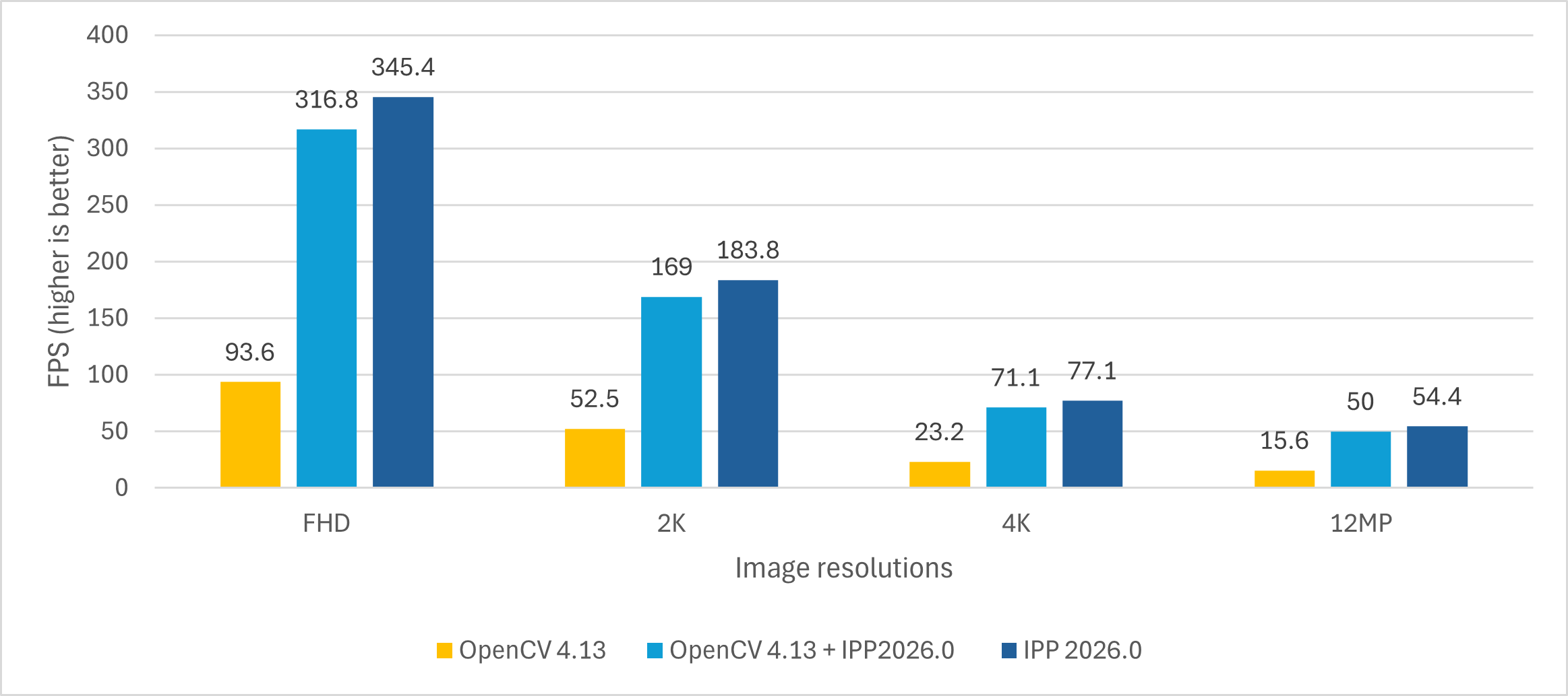
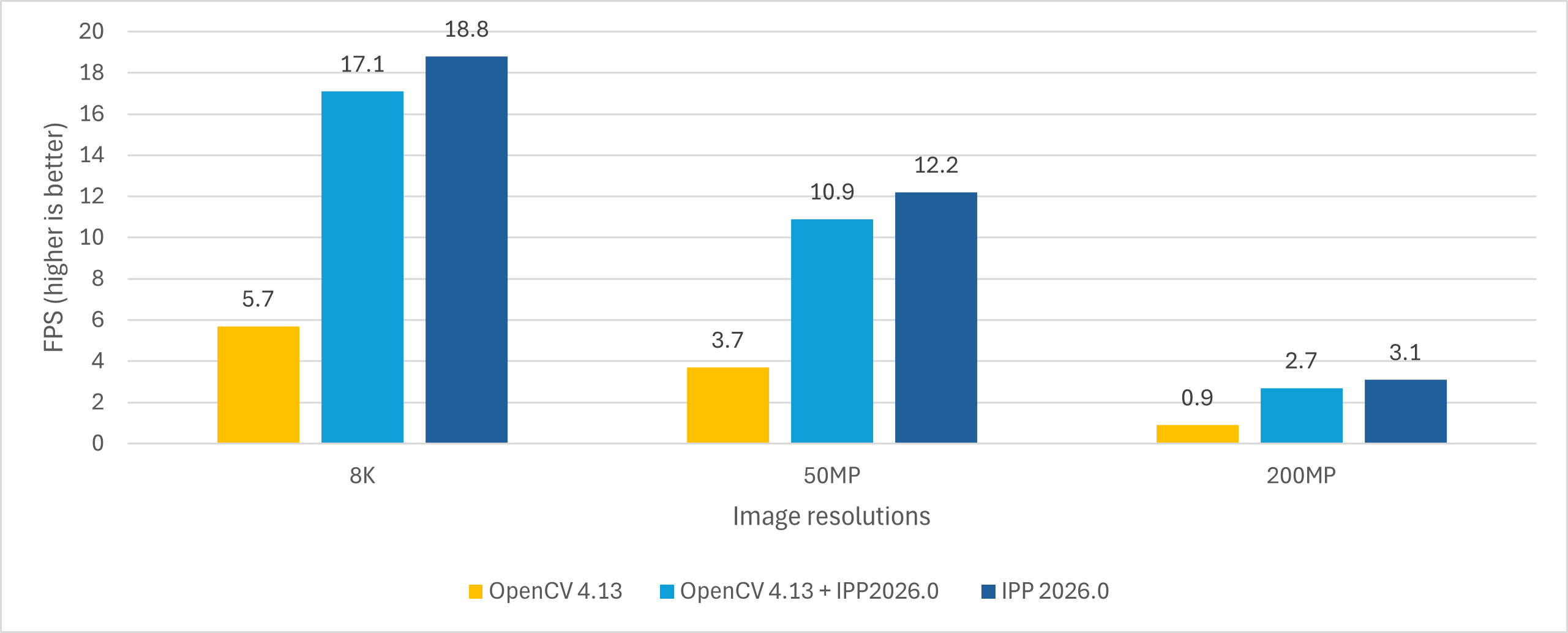
The most popular formats for photos and videos today are 4K and 12MP, so the comparison charts showing the FPS achieved by both libraries are below:
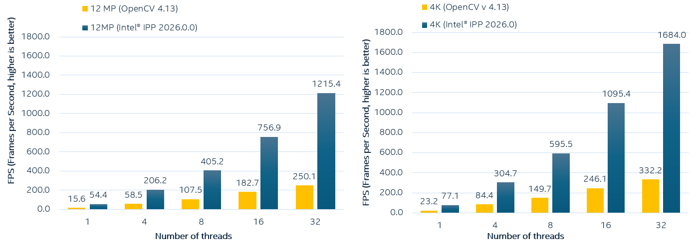
Since our target is 300 FPS on warp operations, let's analyze which computational resources are required for OpenCV and Intel® IPP implementations. The following tables show the warp perspective transformation performance (in FPS) for batch processing of 192 images on Intel® Xeon® 6 processor. We collected the data for 3 implementations (Baseline OpenCV 4.13, OpenCV 4.13 with enforced Intel® IPP calls and Intel® IPP implementation with Cython). The goal of achieving 300 FPS for the pipeline is highlighted in bold:
| Threads | FHD | 2K | 4K | 12MP | 8K | 50MP | 200MP |
|---|---|---|---|---|---|---|---|
| 1 | 93.6 | 52.5 | 23.2 | 15.6 | 5.7 | 3.7 | 0.9 |
| 2 | 178.5 | 100.9 | 44.9 | 30.5 | 11.3 | 7.3 | 1.8 |
| 3 | 255.6 | 144.4 | 65.4 | 44.8 | 16.7 | 10.7 | 2.6 |
| 4 | 326.8 | 183.9 | 84.4 | 58.5 | 21.8 | 14.0 | 3.5 |
| 6 | 432.9 | 252.8 | 119.4 | 83.8 | 31.6 | 20.2 | 4.8 |
| 8 | 577.8 | 313.0 | 149.7 | 107.5 | 40.5 | 25.9 | 6.5 |
| 16 | 999.9 | 495.8 | 246.1 | 182.7 | 70.1 | 43.8 | 11.2 |
| 24 | 912.9 | 568.7 | 301.2 | 226.0 | 89.6 | 55.5 | 14.4 |
| 32 | 1522.0 | 696.2 | 332.2 | 250.1 | 102.3 | 62.9 | 16.4 |
| Threads | FHD | 2K | 4K | 12MP | 8K | 50MP | 200MP |
|---|---|---|---|---|---|---|---|
| 1 | 316.8 | 169.0 | 71.1 | 50.0 | 17.1 | 10.9 | 2.7 |
| 2 | 563.0 | 292.6 | 121.7 | 86.7 | 29.8 | 19.0 | 4.8 |
| 3 | 740.0 | 395.7 | 166.0 | 118.3 | 40.8 | 26.2 | 6.6 |
| 4 | 882.1 | 482.7 | 205.8 | 146.4 | 50.9 | 32.7 | 8.2 |
| 6 | 1102.1 | 619.3 | 276.3 | 194.6 | 68.7 | 44.2 | 11.1 |
| 8 | 1243.4 | 735.4 | 335.2 | 237.4 | 84.0 | 54.3 | 13.5 |
| 16 | 1581.2 | 984.9 | 496.2 | 354.8 | 129.3 | 83.8 | 20.6 |
| 24 | 1816.4 | 1007.4 | 556.4 | 408.6 | 153.4 | 98.9 | 24.4 |
| 32 | 2044.7 | 1050.9 | 590.4 | 440.8 | 171.6 | 110.0 | 26.8 |
| Threads | FHD | 2K | 4K | 12MP | 8K | 50MP | 200MP |
|---|---|---|---|---|---|---|---|
| 1 | 345.4 | 183.8 | 77.1 | 54.4 | 18.8 | 12.2 | 3.1 |
| 2 | 684.1 | 365.4 | 154.1 | 106.5 | 37.6 | 24.1 | 6.1 |
| 3 | 1040.8 | 549.9 | 230.4 | 159.2 | 56.0 | 35.8 | 9.2 |
| 4 | 1377.2 | 731.4 | 304.7 | 206.2 | 73.8 | 46.5 | 12.1 |
| 6 | 2025.3 | 1082.1 | 445.9 | 298.8 | 107.4 | 67.4 | 17.5 |
| 8 | 2735.1 | 1433.2 | 595.5 | 405.2 | 142.9 | 91.3 | 23.9 |
| 16 | 5076.3 | 2568.4 | 1095.4 | 756.9 | 263.4 | 166.8 | 44.4 |
| 24 | 6813.4 | 3464.3 | 1426.3 | 1001.7 | 338.3 | 229.1 | 58.7 |
| 32 | 7558.5 | 4359.7 | 1684.0 | 1215.4 | 420.5 | 279.2 | 72.3 |
Let's compare all three implementations. The OpenCV 4.13 implementation allows achieving 300+ FPS on small resolutions (FHD using 4 threads, 2K using 8 threads, 4K using 24 threads).
The OpenCV 4.13 custom build with enforced Intel® IPP calls for optimized warp perspective performs better, giving almost the same single-thread performance as Intel® IPP, but with lower efficiency when increasing the number of threads due to internal memory allocations. So for 4K it requires more than 16 cores. For 8K, 50MP, and 200MP resolutions, the required FPS is not feasible on 32 threads on the considered CPU.
The Cython version improves the performance significantly, so the required metric is feasible in almost all cases, except 200MP:
- FHD: Achieves 300+ FPS with just 1 thread
- 2K: Achieves 300+ FPS with 2 threads
- 4K: Achieves 300+ FPS with 4 threads
- 12MP: Almost achieves 300+ FPS with 6 threads
- 8K: Achieves 300+ FPS with 24 threads
- 50MP, 200MP: Higher thread counts or alternative approaches needed for 300 FPS target, depending on CPU utilization in the workloads. Usually, using all threads on a NUMA architecture requires special handling, which is out of the scope of this article.
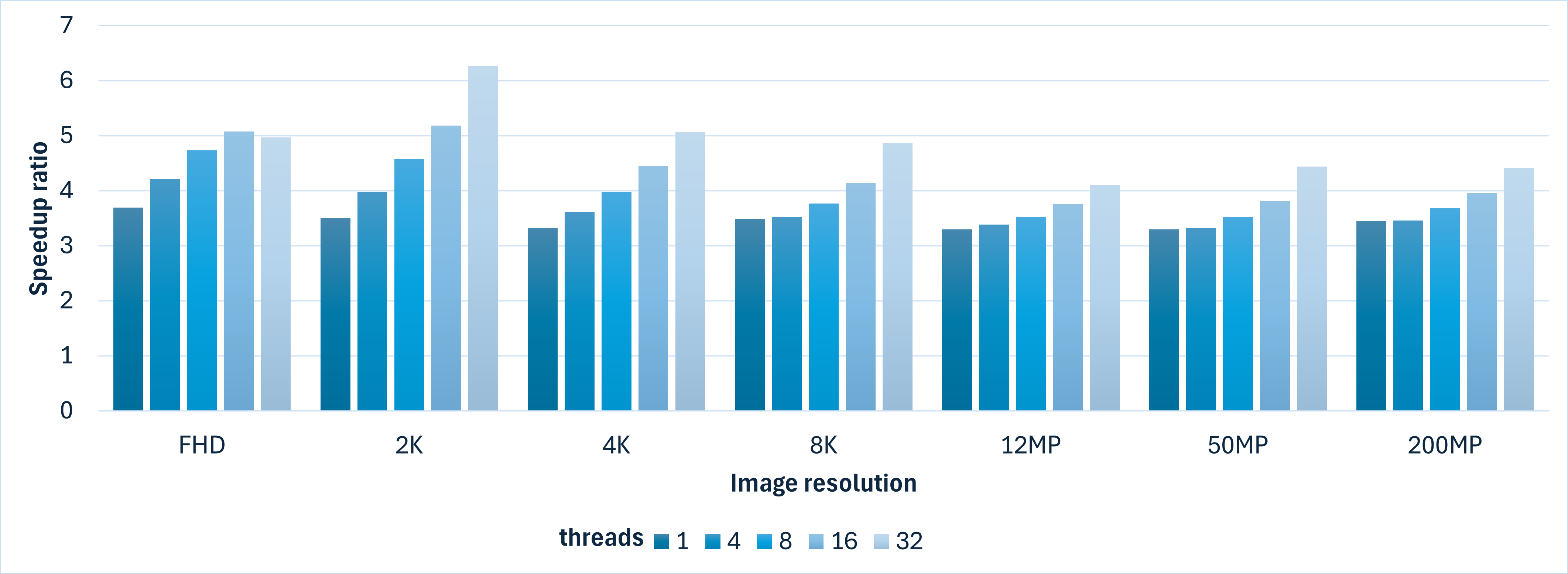
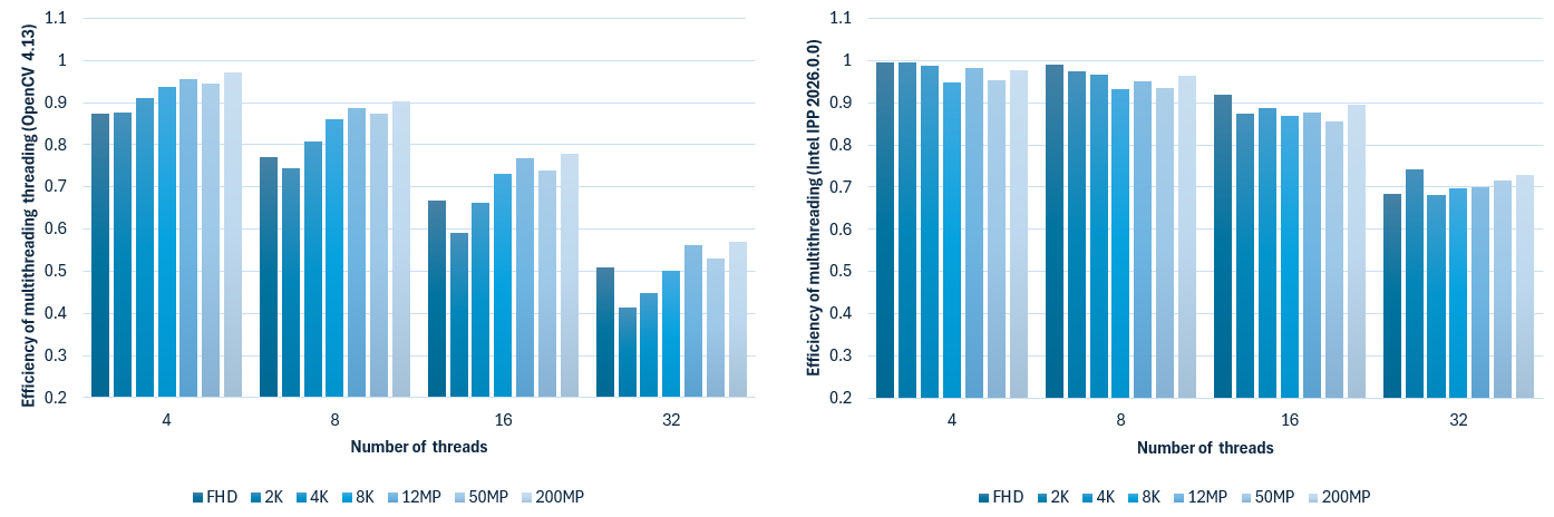
When comparing the efficiency of parallel execution on a single NUMA node, the Intel® IPP-based version performs better and maintains efficiency between 0.9 and 1 for up to 16 threads before dropping to 0.8. OpenCV uses a different threading approach (internal threading) which has lower efficiency, dropping to 0.7 for 32 threads.
The efficiency of threading execution using the OpenCV 4.13 implementation and Intel® IPP 2026.0.0 + Cython.
Conclusion
Both libraries, Intel® IPP 2026.0 and OpenCV 4.13, have their own target use cases. OpenCV remains the most convenient way to work with computer vision in Python, offering an efficient threaded implementation and a ready-to-use Python interface. For many use cases, improved OpenCV performance through Intel® IPP integration is sufficient. This approach works well for warp perspective operations, providing performance improvements at the cost of precision differences between native OpenCV and Intel® IPP implementations, but it requires building OpenCV from source with a custom flag.
When batch execution performance needs to be improved even further, the custom implementation approach using the Intel® IPP library described in this article, or a similar strategy, should be considered. For tuning performance at a lower level, Intel® IPP can provide the required results by enabling efficient problem-specific code design. For the considered batch processing case, the Intel® IPP implementation allows using the minimal required number of threads and minimizing memory allocations. This principle applies broadly to any high-performance Python application that interfaces with native libraries.
References