This is the second tutorial in a three-part series, providing a use case where a credit card company might benefit from machine learning techniques to predict fraudulent transactions.
In part one, you produced a balanced dataset. In this post, you’ll perform some basic transformations on the remaining data to improve the algorithms.
For this tutorial, you’ll need scikit-learn* (sklearn.) It’s a very useful and robust libraries for machine learning in Python*. It provides a selection of efficient tools for machine learning and statistical modeling including classification, regression, clustering, and dimensionality reduction through a consistent interface in Python. This library, which is largely written in Python, is built on NumPy*, SciPy* and Matplotlib*.
The Intel® Extension for scikit-learn offers you a way to accelerate existing scikit-learn code. The acceleration is achieved through patching: replacing the stock scikit-learn algorithms with their optimized versions provided by the extension (see the guide.) That means you don’t need to learn a new library but still get the benefits of using scikit, optimized.
The example below will show the benefits.
Pre-Processing and Transformation
Split data
A common mistake is to perform all the preprocessing transformations on the data before performing the separation between train/test/valid sub-samples. In a real-word case, the data you’ll have available is the training data while test data will be what you’re going to predict. Making the transformation before splitting means that you’ll be transforming the training data with information present in the test dataset, meaning there will be contaminated data and the results will be biased.
How can you avoid it? Simple: by splitting the data. There are multiple ways to do it -- randomly, weighted, among others. Here, you’ll divide it randomly, but with balanced examples of both classes (50/50 if possible.) It’s good practice to divide in a 80/20 ratio, meaning that 80% of our data will be used to train the model (there’s a validation dataset which could be the 20% of the train data, this is useful when training the model to see how it’s performing), and 20% will be used to verify how the model performs with data the model has never seen before.
In short, we could use the whole dataset to visualize it, but it needs to be split up as soon as you start working on transformations.
Transformations
Now you’ll modify the data to make it easier for the algorithm to detect its behavior. These are the most common transformations, and even so they require patience. After training the model you’ll find out if these transformations were useful or not. You can train a model without any transformation, but it’s highly recommended to transform the data first.
A transformation can be understood as a modification of the data without changing its patterns. For example, if you have a feature called “age” represented in values between 0 and 100, it might be represented in groups such as young (0), adult (1), senior (2.)
Scaling
It's always a good idea to scale the data to reduce the effect of data represented in value ranges. The model might skew towards those features with bigger numbers, for example if “customer seniority” is represented from 0-20 and the “transaction amount” is between 1,000 and 10,000,000, the model might weight the “transaction amount” more than customer seniority. Which might be true, but you’ll be biased if the model is trained with data in this format.
X_train.describe()

As you can see from the train data output, most of the features give us the impression that are “scaled” except for “time” and “amount,” which have larger numbers. Avoid using the data as it is now because the model would interpret “time” and “amount” as the two most important features.
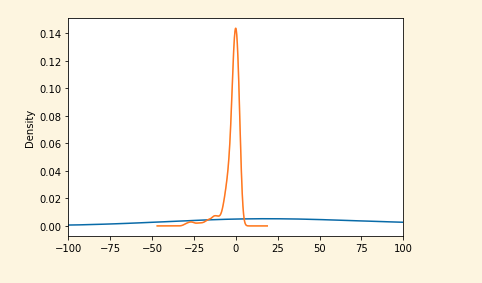
If you plot amount and a feature (V1, orange), you'll notice that amount (blue) appears much lower and not centered at all. This happens because the values of V1 and amount are very different, and it will affect how our model can learn from those features.
X_train['Amount'].plot(kind='kde',xlim=(100,100))

X_train['V1'].plot(kind='kde',xlim=(-100,100))

Let’s scale the data now. The idea is to keep the same “smaller” distribution, representing the initial data between the same defined range to all features.
There are multiple tools and options to scale and you can do it manually, but scikit-learn* has an API to help with this task. It will depend on the data we have (here’s a good guide to select useful calculations).
In our example we’ll scale the data, using the StandardScale function (industry’s go-to algorithm), you can try others as RobustScaler. StandardScaler means that each feature will have a mean of 0, and each value is divided by the standard deviation. Your goal is to try to center the distribution of the data to reduce the effect of variables that are in a different scale. Note that if our data has outliers (as explained below), we should try to reduce the effect by using other scalers like RobustScaler.
standard = StandardScaler()

data_st = standard.fit_transform(X_train)   # This function gives the data as an array


# convert the array back to a dataframe
dataset_std = DataFrame(data_st, columns=col_names)   #The col_names was extracted when StandardScaler converted the dataset

dataset_std.describe()

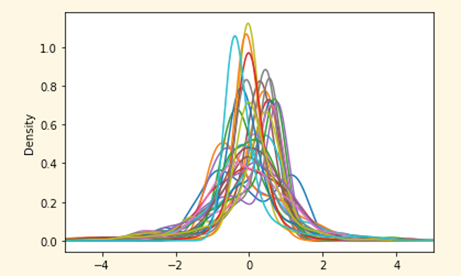
As we can see after using the StandarScaler all features are centered at 0. More importantly, the model can now “see” the behavior of all features.

Outliers
Now that the data is almost ready to train our model, there’s another important thing to check. It’s well organized now but we can still find values in the features (columns) that can affect the model as it might be the presence of an outlier.
An outlier is a value whose distance from other values is abnormal (unusual.) For example, if most customer transactions (the mean) cluster around a value, let’s say $100. An outlier is a transaction of $1 million and using this value to train our model will have a negative effect because it misleads the training process resulting in longer training times, less accurate models, and ultimately poorer results.
Therefore, you need to know how to handle these values, whether they are mild or extreme. Outliers should be carefully investigated. They often contain valuable information about the process under investigation or the data gathering and recording process -- an error might add extra numbers and make the value appear as an outlier. Before considering removal, try to understand why they appeared and whether similar values are likely to continue to appear. Of course, outliers are often bad data points.
In this example, you’ll eliminate those values that are three times away from interquartile range (the difference between 25% and 75% of the data), which are called extreme outliers (1.5 of distance are regular outliers), since you are not able to understand the data (it’s anonymized, and we don’t know how the data was extracted.) To identify them, you can use two graphic techniques, box plots and scatter plots.
Here’s an example, keeping in mind that in real-case scenario with more information about the features you could investigate further.
# Example to plot the outliers for 1 feature. You'll be using V5

fig = plt.figure(figsize =(10,5))


# Creating plot
plt.boxplot(X_train['V1'].loc[X_train['Class'] == 1],whis=3)    # "whis" is to define the range of IQR, you’ll only find extreme values on FRAUD class

# show plot
plt.show()

## # Example to plot the outliers for 1 feature

# # V1

v1_fraud = X_train['V1'].loc[X_train['Class'] == 1].values

q25, q75 = np.percentile(v1_fraud, 25), np.percentile(v1_fraud, 75)

print('Quartile 25: {} | Quartile 75: {}'.format(q25, q75))

v1_iqr = q75 - q25

print('iqr: {}'.format(v1_iqr))


v1_cut_off = v1_iqr * 3

v1_lower, v1_upper = q25 - v1_cut_off, q75 + v1_cut_off

print('Cut Off: {}'.format(v1_cut_off))

print('V5 Lower: {}'.format(v1_lower))

print('V5 Upper: {}'.format(v1_upper))


outliers = [x for x in v1_fraud if x < v1_lower or x > v1_upper]


print('Feature V5 Outliers for Fraud Cases: {}'.format(len(outliers)))

print('V5 outliers:{}'.format(outliers))
Quartile 25: -0.6759968729894883 | Quartile 75: 0.3525708873721557 iqr: 1.028567760361644
Cut Off: 3.0857032810849323
V5 Lower: -3.7617001540744206 V5 Upper: 3.438274168457088
Feature V5 Outliers for Fraud Cases: 15
V5 outliers:[-4.34089141951856, -4.939504436487541, -4.435575709837507, -4.435575709837507, -4.849268706743759, -4.319494204359201, -4.435575709837507, -5.06372102689204, -4.0924369554578055, -4.765817290040161, -4.815283422793271, -3.968200713661824, -3.8439577145416677, -3.9811813282975925, -4.691057645556144]
Now you can remove those outliers. Remember to do this process only once, because each time you do it you’ll uncover new outliers and reduce the dataset.
Next, take a look at those values. You’ll need to iterate through all the features to remove extreme outliers in each one.
# Let's remove the outliers

for feature in X_train.columns.difference(['Class']):      # Loop into each feature except class


    feature_fraud = X_train[feature].loc[X_train['Class'] == 1].values

    q25, q75 = np.percentile(feature_fraud, 25), np.percentile(feature_fraud, 75)

    feature_iqr = q75 - q25


    feature_cut_off = feature_iqr * 3

    feature_lower, feature_upper = q25 - feature_cut_off, q75 + feature_cut_off


    outliers = [x for x in feature_fraud if x < feature_lower or x > feature_upper]


    X_train = X_train.drop(X_train[(X_train[feature] > feature_upper) | (X_train[feature] < feature_lower)].index)


print('Number of Instances after outliers removal: {}'.format(len(X_train)))
Number of Instances after outlier’s removal: 652
As you can see, our dataset is reduced but there’s still enough to train your model. This is not a 50/50 ratio anymore. You can divide again to get 50/50 if you want. However, 57/42 is still a good ratio between FRAUD and NO FRAUD cases.
print('No Frauds', round(X_train['Class'].value_counts()[0]/len(X_train) * 100,2), '% of the dataset')

print('Frauds', round(X_train['Class'].value_counts()[1]/len(X_train) * 100,2), '% of the dataset')
No Frauds 57.82 % of the dataset
Frauds 42.18 % of the dataset
Feature engineering
Lastly, there’s another important modification to make to your dataset. Feature engineering (FE) or means adding features that are not present and to help the algorithm detect patterns in data. Data scientists call it an art because you need to figure out which feature can be added to help and it involves deep understanding of the data. It’s a process of trial and error; don’t worry if that new feature doesn’t work when you test the results. Auto machine learning (AutoML) tools can help. They automatically test parameters so you can find “optimal” feature combinations that can also be used during training.
For example, if you know the description of each feature, suppose there are two features called “amount” and “age.” You could create a new feature called “amount spent by age,” then create a function that splits age ranges and hashes them based on the amount spent. In some cases, it can also just be a categorical value. Here, the data is anonymized so adding features is tricky, but it’s important to be aware of FE.
Conclusion
In this tutorial, we highlighted the most important preprocessing techniques to use on a tabular data problem such as our fraud detection case.
Now your data is ready to be used to train a model (Part three.) The preprocessing and training stages are an iterative process in which transformations performed may or may not help teach the algorithm. Remember that your goal is to have an algorithm that can work well on unseen data in the very last stage. You might have to repeat or modify this process several times to get there.
Stay tuned for Part three!
About the author
Ezequiel Lanza, Open Source Evangelist
Passionate about helping people discover the exciting world of artificial intelligence, Ezequiel is a frequent AI conference presenter and the creator of use cases, tutorials, and guides that help developers adopt open source AI tools like TensorFlow* and Hugging Face*. Find him on Twitter at @eze_lanza