Frederico L. Cabral – fcabral@lncc.br
Carla Osthoff – osthoff@lncc.br
Marcio Rentes Borges – marcio.rentes.borges@gmail.com
National Laboratory for Scientific Computing (LNCC)
Introduction
In order to exploit the capabilities of parallel programming in many-core processor architecture that is present in the Intel® Xeon Phi™ coprocessor, each processor core must be used as efficiently as possible before going to a parallel OpenMP* approach. Otherwise, increasing the number of threads will not present the expected speedup. In this sense, the so-called “top-down characterization of micro-architectural issues” should be applied1.
In this paper, we present some analysis for potential optimization for a Godunov-type semi-discrete central scheme, proposed in2, for a particular hyperbolic problem implicated in porous media flow, for Intel® Xeon® processor architecture, in particular, the Haswell processor family which brings a new and mode advanced instruction set to support vectorization. This instruction set is called Intel® Advanced Vector Extensions 2 (Intel® AVX2), which follows the same programming model that its previous Intel AVX family used and at the same time extends it by offering most of the 128-bit SIMD integer instructions with 256-bit numeric processing capabilities3.
Considering the details in this architecture, one can achieve optimization and obtain a considerable gain of performance even in single-thread execution before going to parallelization approach. The auto-vectorization followed by semi-auto vectorization permits the extraction of the potential for one thread which will be crucial for the next, parallelization step. Before using more than one single thread it's to be sure that a single thread is executed efficiently.
This paper is organized as follows: section 2 explains what a porous media application is and how it's important to oil and gas recovery studies; section 3 explains the numerical method used in this analysis for a hyperbolic problem; section 4 describes the hardware and software environment used in the paper; section 5 explains optimization opportunities and results; section 6 shows the results for some different sizes of the problem; section 7 analyzes the OpenMP parallel approach and Intel® Advisor analysis; section 8 presents the conclusion and future work.
Porous Media Flow Application
As mentioned in2 “In porous media applications, flow and transport are strongly influenced by spatial variations in permeability and porosity fields. In such problems, the growth of the region, where the macroscopic mixing of fluids occurs, is dictated by rock heterogeneity acting in conjunction with fluid instabilities induced by unfavorable viscosity ratio. Usually, one assumes heterogeneity solely manifested in the permeability field with porosity commonly assumed homogeneous 1 - 3 or inhomogeneous but uncorrelated with the permeability4. However, as deeper reservoirs are detected and explored, geomechanical effects arising from rock compaction give rise to time-dependent porosity fields. Such phenomenon acting in conjunction with the strong correlation between permeability and porosity somewhat affects finger growth, leading to the necessity of incorporating variability in porosity in the numerical modeling. In the limit of vanishing capillary pressure, the fluid-phase saturations satisfy a hyperbolic transport equation with porosity appearing in the storativity term. Accurate approximations of conservation laws in strongly heterogeneous geological formations are tied up to the development of locally conservative numerical methods capable of capturing the precise location of the wave front. Owing to the fact that the saturation entropy solutions admit nonsmooth composite waves.”
Numerical Method for a Hyperbolic Problem
The numerical method used in this paper is devoted to solving the following partial differential equation.
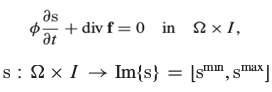
Where 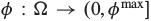 is the storage coefficient and is a scalar function, and the vector
 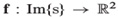 represents a flux of the conserved quantity s, which may depend on other functions of position and time (for example, on Darcy velocity in porous media applications)2.
Experiment Environment
All tests presented herein were executed in a 14.04 Ubuntu* computer with an Intel® Core™ i5-4350U processor @ 1.40 GHz with two real cores and hyper-threading (a total of four simultaneous threads). This processor belongs to the Intel Haswell family that has full support of Intel® Advanced Vector Extensions 2 (Intel® AVX2), which is the focus of this paper. This computer has 4 GB of RAM and 3 MG of cache. Intel® Parallel Studio XE 2015 was used to analyze performance and guide toward the optimization process.
Optimization Opportunities
This section presents the analysis and identifies the parts inside the code that can permit optimization via vectorization and parallelization. To accomplish that, Intel tools such as Intel® VTune™ Amplifier, Reports generated by Compiler, and Intel® Advisor are used. Such tools perform some kinds of analysis inside the source and binary (executable) code and give hints on how to optimize the code. This task is mostly applied to performance bottlenecks analysis inside the CPU pipeline. Modern CPUs implement a pipeline together with other techniques like hardware threads, out-of-order execution, and instruction-level parallelism to use hardware resources as efficiently as possible1. The main challenge for an application programmer is to take full advantage of these resources, because they rely on the microarchitecture level, which is “far distant” from the programming level available in modern and widely used programming languages such as C, C++, and Fortran*.
Intel tools can help by analyzing compiler/linker and execution times to identify how those resources are being used. First, the compiler is able to inform a report where one can discover what was automatically done and what was not, for optimization goals. Sometimes a loop will be vectorized and other times it will not, and in both cases the compiler tells that and it's useful to the programmer to know whether an intervention is needed or not. Second, Intel VTune Amplifier shows the application behavior in the pipeline and on the memory usage. It’s also possible to know how much time is spent in each module and whether the execution is efficient or not. Intel VTune Amplifier creates high-level metrics to analyze those details, such as cycles-per-instruction, which is a measure of how fast instructions are being executed. Finally, Intel Advisor can speculate and tell how much performance can be improved with thread parallelism. By combining all these tips and results, the programmer is able to make changes in the source code as well as in compiler options to achieve the optimization goal.
Auto Vectorization
Recent versions of compilers are able to vectorize the executable code by setting the optimization compiler option to O2 or higher. One can disable vectorization by using the -no-vec compiler option, which can be helpful to compare results. Briefly, vectorization is the ability of perform some operations in multiple data in a single instruction5. Let’s take the following loop as an example.
for (i=0; i<=MAX; i++) {
       c[i] = b[i] + a[i];
}
If this loop is not vectorized, in memory registers it will look something the image shown in Figure 1.
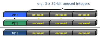
Figure 1: Non-vectorized piece of code.
The same loop can be vectorized (see Figure 2), and the compiler may use the additional registers to perform four additions in a single instruction. This approach is called Single Instruction Multiple Data (SIMD).
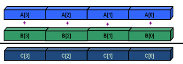
Figure 2: Vectorized loop.
This strategy often leads to an increase in performance as one instruction operates simultaneously on more than one data.
In the flow application studied in this paper, the auto-vectorization presents a speedup of two times over a Haswell processor that has an Intel AVX2 instruction set. The -xHost option instructs the compiler to generate code according to the computer host architecture. In the case of a Haswell host, this option will guarantee that Intel AVX2 instructions are generated. Figure 3 shows the Intel VTune Amplifier summary where the elapsed time is 186.628 seconds, Clocks per Instruction (CPI) about 0.5, and a total number of 1.067.768.800.000 instructions retired.
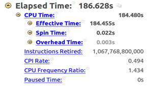
Figure 3: Intel® VTune™ Amplifier summary without xHost.
The main goal of optimization is to reduce the elapsed time and increase CPI, which should be ideally 0.75—full pipeline utilization.
Figure 4 shows the top-down tree ordered by effective time by utilization for each module in the application. Note that the function “vizinhanca” is the most expensive, consuming about 20 percent of the total time. This function computes porosities, permeabilities, velocities, flux on the element, and the flux on all neighboring elements for all elements at the mash on mass calculation step.
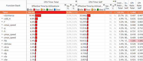
Figure 4: Top-down tree.
Notice that CPI is critically poor for the “fkt” function that computes flux at a given time step, for all steps. This function calls “vizinhanca”.
Figure 5 shows part of the “vizinhanca” source code, the time to execute each line, and the corresponding assembly code for the selected line, which computes the linear reconstruction. Notice that the instructions generated are not specifically the Intel AVX2 instructions.
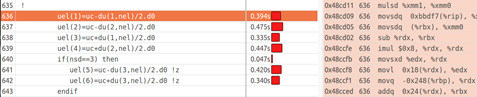
Figure 5: Assembly code for linear reconstruction.
The instructions MULSD, MOVSDQ, SUB, IMUL, MOVSXD, MOVL, MOVQ, and ADDQ are all from the Intel® Streaming SIMD Extensions 2 (Intel® SSE2) instruction set. These “old” instructions were released with the Intel® Pentium® 4 processor in November 2000.
Compiling the same code with -xHost, which instructs the compiler to generate code for the host architecture, and executing via Intel VTune Amplifier, the total elapsed time is reduced to 65.657 seconds with CPI Rate equal to 0.628, which is much better and closer to the ideal 0.75 value (see Figure 6).
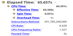
Figure 6: Intel® VTune™ Amplifier summary with xHost.
To understand why it happens, one can look at the assembly code and notice that instructions are generated for Intel AVX2. It's also noticed that the Instructions Retired metric is much smaller than the non-vectorized version. This occurs because the metric does not count instructions that were canceled because they were on a path that should not have been taken due to a mispredicted branch. Thus the total amount of mispredict is much smaller, which also explains the increase of CPI [7]. Figure 7 shows the same piece of code as shown in Figure 5. Notice that most of the assembly instructions are Intel AVX2 instead of Intel SSE2. The difference is due to the mnemonic for each instruction, where the prefix V as in VMOV instead of MOV means it's a vector instruction.
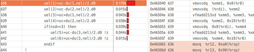
Figure 7: Assembly vectorized code for linear reconstruction.
Figure 8 shows the differences among registers for the Intel SSE2, Intel AVX, and Intel AVX2 instructions sets6.
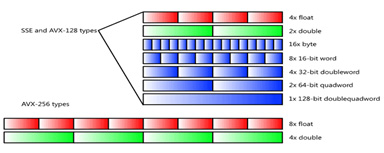
Figure 8: Registers and instruction set.
This simple auto-vectorization permitted a gain in performance of up to three times faster.
Identifying other Hotspots
Considering that four threads can be executed by two physical cores and only optimizations made so far regards on compiler auto-vectorization, there is room for more optimization and to achieve that, bottlenecks need to be recognized. The original source code of the Flow Application has many lines with division instead of multiplying by the inverse.
The -no-prec-div option instructs the compiler to change division by inverse multiply, and its use has been shown to improve performance of the Flow Application.
Figure 9 shows a piece of source code where division is widely used. The code is inside the “udd_rt function”, one the bottlenecks of the code, according to analysis presented in Figure 4.
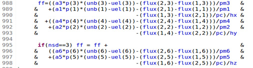
Figure 9: Many divisions in a critical piece of code.
The use of -no-prec-div has one problem: according to5 sometimes the value obtained is not as accurate as IEEE standard division. If it is important to have fully precise IEEE division, use this option to disable the floating-point division-to-multiplication optimization, leading to a more accurate result, with some loss of performance.
Another important issue that Intel can support is the fact that the flow application has a significant number of modules in Fortran which can be a challenge to optimization. To guarantee the optimization of inter-procedures the -ipo option instructs the compiler and linker to perform Interprocedural Optimization. Some part of the optimization is left to the linker phase.
With the use of -ipo, -xHost, and -no-prec-div, the total elapsed time is reduced even more, according to Figure 10.
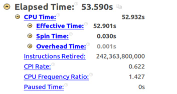
Figure 10: ipo, xHost and no-prec-div options.
To better understand the role of -no-prec-div, a test without it was executed and the total elapsed time increased to 84.324 seconds, revealing that this option is responsible for a gain of about 1.5 times faster. Another test without the -ipo option led to an elapsed time equaling 69.003 seconds, revealing a gain of about 1.3 times faster.
Using Intel® VTune™ Amplifier General Exploration to Identify Core and Memory Bounds
Intel VTune Amplifier does more than inform elapsed time, CPI, and instructions retired. Using General Exploration it’s possible to obtain information about program behavior inside the CPU pipeline, revealing where performance can be improved by detecting core and memory bounds. Core bound refers to issues that are unrelated to memory transfer and affect performance in out-of-order execution or saturating some execution units. Memory bound refers to fractions of cycles where pipeline could be stalled due to demand load/store instructions. Combined, these two metrics define the so-called back-end-bound, which combined with the front-end-bound inform stalls that cause unfilled pipeline slots.
A typical modern out-of-order pipeline is shown in Figure 11, which identifies two different parts: front-end and back-end1.
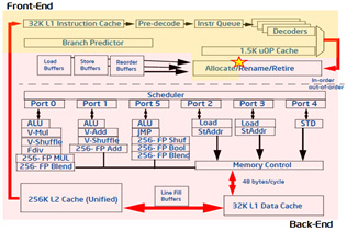
Figure 11: Out-of-order Intel CPU pipeline.
At the back-end part are the ports to deliver instructions to ALU, Load, and Store units. Unbalanced utilization of those ports will in general negatively affect the whole performance, because some of execution units can be idle or used less frequently while others can be saturated.
For the application studied herein, this analysis showed that even with the auto-vectorization by the compiler, there's still some core bound due to unbalanced instruction dispatches among the ports.
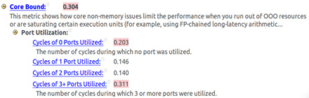
Figure 12: Core bound.
Figure 12 shows there was a high rate 0.203, which means 20.3 percent of clock cycles had no ports utilized, meaning poor utilization. Also there was a high rate 0.311, meaning 31.1 percent of cycles had three or more ports utilized, which caused saturation. Clearly there is unbalanced port utilization.
In the bottom-up Intel VTune Amplifier analysis presented in Figure 13, it’s possible to identify the causes of core bound mentioned above. In this case the Intel VTune Amplifier indicates a high back-end bound in four functions (fkt, udd_rt, xlo, and xmax_speed) in the program and in the “transport” module. A high rate of bad speculation is also detected for the “xmax_speed” function.
The next step for using Intel VTune Amplifier as a tool to analyze those issues involves looking into each function in order to identify pieces of code where time (clock cycles) is being wasted.
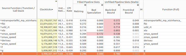
Figure 13: Back-end bound.
By analyzing each function that appears in the back-end bound, it’s possible to identify where those bounds occur. As shown in Figures 14–17, Intel VTune Amplifier exhibits the source code with corresponding metrics for each line, such as retiring, bad speculation, clockticks, CPI, and back-end bound. In general, a high value of clockticks indicates the critical lines in the code, which Intel VTune Amplifier exhibits by highlighting the correspondent value.
In the “transport” function, there is a high bound as shown in Figure 14.
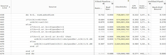
Figure 14: Back-end bound in transport function.
The “fkt” function seams to be critical since it calls the “g” and “h” functions to compute flux and the “udd_rt” function to compute saturation on the anterior element of the mesh as can be observed at the piece of code analyzed in Figure 15.
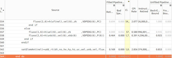
Figure 15: Back-end bound in fkt function.
Functions “f” and “g” called by “fkt” are listed below.
function g(uu,vv,xk,VDISPY,POROSITY)
!
!	computes f in a node or volume
!
use mPropGeoFisica, only: xlw,xlo,xlt,gf2,rhoo,rhow

implicit none
real(8) :: g,uu,vv,xk
REAL(8) :: VDISPY,POROSITY
real(8) :: fw
real(8) :: xlwu,xlou
real(8) :: xemp,xg

xlwu=xlw(uu)
xlou=xlo(uu)
fw=xlwu/(xlwu+xlou)
xg = gf2
xemp=fw*xg*xlou*xk*(rhoo-rhow)
g=fw*vv-xemp

end function

function h(uu,vv,xk,VDISPZ,POROSITY)
!
!	computes f in a node or volume
!
use mPropGeoFisica, only: xlw,xlo,xlt,gf3,rhoo,rhow

implicit none
real(8) :: h,uu,vv,xk
REAL(8) :: VDISPZ,POROSITY
real(8) :: fw
real(8) :: xlwu,xlou
real(8) :: xemp,xg

xlwu=xlw(uu)
xlou=xlo(uu)
fw=xlwu/(xlwu+xlou)
xg = gf3
xemp=fw*xg*xlou*xk*(rhoo-rhow)
h=fw*vv-xemp

end function
It's important to emphasize that “f” and “g” are 2D components of vector F, which represents a flux of conserved quantity “s” according to

Function “xlo” that computes total mobility according to water and oil mobilities, presents a high back-end bound too, according to Figure 16.
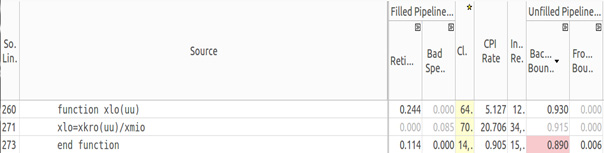
Figure 16: Function xlo.
Figure 17 shows the function “xmax_speed” that computes the maximum speed in the x direction. “xmax_speed” is the other function responsible for the high back-end bound.
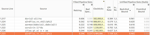
Figure 17: Function xmax_speed.
Intel VTune Amplifier uses the four functions presented above—“transport”, “fkt”, “xlo,” and “xmax_speed”—to indicate back-end bound.
Back-end bound can be caused by core or memory bound. Once the auto-vectorization has been already performed, it's highly probable that the results shown above are caused by memory issues (see Figure 18). Indeed, Intel VTune Amplifier indicates some L1 cache bound.
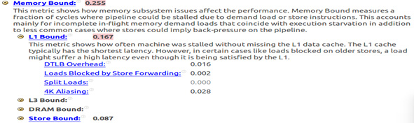
Figure 18: Memory bound.
Once this application has a great number of data structures, such as vectors, that are necessary in many different functions, they must be studied in detail to identify actions to improve performance by reducing this memory latency. The issue of data alignment must also be considered in order to assist vectorization4.
Using Compiler Reports to Identify More Hints and Opportunities
In order to identify more opportunities to optimize the code via vectorization, a compiler report should be used because it gives hints about potential vectorizable loops. The MTRANSPORT module becomes the focus of analysis once computational effort is concentrated there.
Some outer loops are not vectorized because the corresponding inner loop is already vectorized by the auto-vectorization approach, which was explained previously. The compiler message for this case is:
remark #####: loop was not vectorized: inner loop was already vectorized
In some cases the compiler instructs the programmer to use a SIMD directive, but when this is done, the loop cannot be vectorized because it performs an assignment to a scalar variable, as shown in the following loop.
!DIR$ SIMD
      do n=1,nstep+1
      ss=smin+(n-1)*ds
The corresponding compiler message is
LOOP BEGIN at ./fontes/transporte.F90(143,7)
     remark #15336: simd loop was not vectorized: conditional
     assignment to a scalar   [ ./fontes/transporte.F90(166,23) ]
     remark #13379: loop was not vectorized with "simd"
Most parts of loops were vectorized automatically by the compiler, and in some cases the potential speedup estimated by the compiler varies from 1.4 (most of them) to 6.5 (only one).
When the compiler detects that vectorization will produce a loss of performance (a speedup of less than 1.0), it doesn't perform vectorization. One example is shown below.
LOOP BEGIN at ./fontes/transporte.F90(476,7)
      remark #15335: loop was not vectorized: vectorization
		possible but seems inefficient. Use vector always directive
		or -vec-threshold0 to override
      remark #15451: unmasked unaligned unit stride stores: 1
      remark #15475: --- begin vector loop cost summary ---
      remark #15476: scalar loop cost: 3
      remark #15477: vector loop cost: 3.000
      remark #15478: estimated potential speedup: 0.660
      remark #15479: lightweight vector operations: 2
      remark #15481: heavy-overhead vector operations: 1
      remark #15488: --- end vector loop cost summary ---
LOOP END
The real speedup obtained with auto-vectorization is about three times, according to compiler estimated mean value.
Analyzing the reasons that the compiler didn't vectorize some loops should be considered before performing more optimizations on the application.
Experiments with Other Grid Sizes
All tests made up to this point were executed with a 100×20×100 mesh that computes 641 transport steps with one thread.
In this section other sizes of mesh will be considered in order to compare the total speedup obtained via auto-vectorization. Table 1 shows this comparison.
| Mesh |
Time without Vectorization |
Time with Vectorization |
Speedup |
Number of Transport Steps |
|---|---|---|---|---|
| 100×20×100 | 186,628 | 53,590 | 3,4 | 641 |
| 50×10×50 | 17,789 | 5,277 | 3,4 | 321 |
| 25×5×25 | 0,773 | 0,308 | 2,5 | 161 |
| 10×2×10 | 0,039 | 0,0156 | 2,5 | 65 |
Table 1: Comparison of total speedup obtained using auto-vectorization.
These tests show the tendency of speedup to be achieved with auto-vectorization as it is greater the bigger the mesh is. It's an important conclusion because real problems require more refined (bigger) meshes.
In further phases of this project, more refined meshes need to be considered to validate this hypothesis.
Parallel OpenMP* multithread approach
Once semi-auto vectorization is achieved, it's possible to investigate how fast the application can become when executed with more than a single thread. For this purpose, this section presents an initial experiment comparing the analysis via Intel VTune Amplifier with one and two threads.
The tests described herein were performed in a different machine than the one described in section 4. For this section seven tests were executed in a 14.04.3 LTS Ubuntu computer with a Intel® Core™ i7-5500U processor @ 2.40 GHz with two real cores and hyper-threading (a total of four simultaneous threads). This processor belongs to the Intel Broadwell family that has full support of Intel AVX2. This computer has 7.7 GB of RAM and 4 MG of cache. Intel Parallel Studio XE 2016 was used to analyze performance and guide toward the optimization process. Broadwell is Intel's codename for the 14-nanometer die shrink of its Haswell microarchitecture. It is a "tick" in Intel's tick-tock model as the next step in semiconductor fabrication.
The first test was executed in a single thread and with the -ipo, -xHost and -no-prec-div compiler options, just like in section 5.2. The same 100×20×100 mesh that executes 641 transport steps took 39.259 seconds, which means a gain about 1.4 times faster than the result obtained with the Haswell processor as described in section 6, Table 1. Figure 19 shows part of the Intel VTune Amplifier summary for this case.
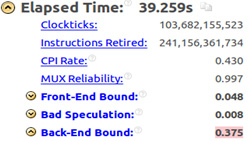
Figure 19: Intel® VTune™ Amplifier summary.
An important issue to be considered is that with a processor that is 1.7 times faster, the gain obtained was just 1.4, which suggests that the microarchitecture resources are not being efficiently used. The Intel VTune Amplifier summary presented in Figure 19 shows a back-end bound equal to 0.375 suggesting that even by increasing clock frequency the causes of some bounds may not be solved.
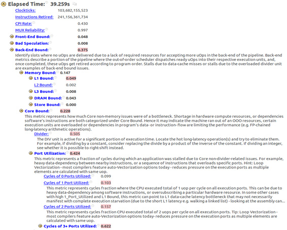
Figure 20: Intel® VTune™ Amplifier analysis.
Figure 20 shows that there is a high back-end bound due to a core bound that is caused by the divider unit latency. There are other core issues unrelated to the divider unit referred as "Port Utilization” in VTune. This “Port Utilization" metric indicates how much efficient execution ports inside ALU are used. As cited in8, core bound is a consequence of the demand on the execution units or lack of Instructions-Level-Parallelism inside the code. Core bound stalls can manifest among other causes, because sub-optimal execution port utilization. For example, a long latency divide operation might serialize execution, increasing the demand for an execution port that serves specific types of micro-ops and as a consequence it will cause a small number of ports utilized in a cycle.
It indicates that the code must be improved in order to avoid data dependencies and a more efficient vectorization approach beyond the semi-auto vectorization applied so far.
Figure 21 shows the Intel VTune Amplifier bottom-up analysis where the parts of the code are identified as the cause of back-end bound, which are the same that were identified in section 5.3, Figure 13.
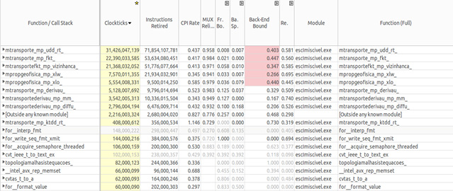
Figure 21: Intel® VTune™ Amplifier bottom-up analysis.
It's possible to conclude that even by increasing the CPU clock frequency the bottlenecks tend to remain the same or eventually appear in new regions of the code, because of the out-of-order execution and the faster demand to computational resources.
Two OpenMp Threads
It's crucial to analyze the impact of parallelism in the speedup for this application with two and more OpenMP multi-threads. Since the hardware available has two real cores with hyper-threading, tests were made with two threads to compare how a real core can contribute to reducing execution time.
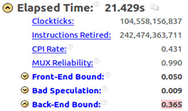
Figure 22: Intel® VTune™ Amplifier summary analysis.
Figure 22 shows an Intel VTune Amplifier summary analysis for the similar case presented in the previous section with the only difference being that the OMP_NUM_THREADS environment variable was set to 2. The gain is about 1.8 times faster but still has a high back-end bound due to the reasons explained before.
Figure 23 shows the same bottlenecks and in addition a bad speculation in the “xlo” function and a high retiring rate in the “xlw” function.
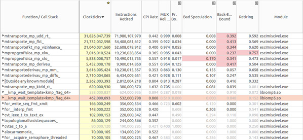
Figure 23: Intel® VTune™ Amplifier bottom-up analysis.
According to8, a bad speculation indicates that slots are wasted due to wrong speculation that can be cause by two different reasons: (1) slots used in micro-ops that eventually don’t retire, and (2) slots in which the issue pipeline was blocked due to recovery from earlier mis-speculations. When the number of threads is increased the data dependencies between them starts to happen, which can cause mis-speculations that are speculations discarded during out-of-order pipeline flow. The increase in retire rate for the “xlw” function indicates that parallelism improved the slot utilization, even slightly.
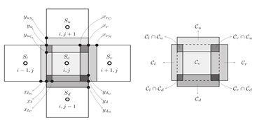
Figure 24: Finite Element Mesh.
Figure 24 shows the stencil used in the numerical method, which leads to a data dependence between threads in the parallel approach. Each element “O” in the mesh used by the numerical method depends on data coming from its four neighbors: left, right, up, and down. The light gray indicates the regions in the mesh that are shared between the element and the neighbors. The dark gray indicates the regions that are shared among the element itself and the other two neighbors. The points xl, xln, xlc, xr, xrn, xrc, yun, yu, yuc, ydc, yd and ydn are points shared among adjacent elements and here show the possible bottleneck for a parallel approach, since data must be exchanged among parallel threads, and synchronization methods need to be implemented via OpenMP barriers in the transport module.
In order to verify whether the size of the problem affects the parallel speedup, other mesh sizes were tested and no significant differences were observed for smaller meshes (see Table 2), except for the 10×2×10 mesh which presents a very low workload. The OpenMP overhead for creating and destroying threads is also a limiting factor.
| Mesh |
Time with One Thread |
Time with Two Threads |
Speedup |
Number of Transport Steps |
|---|---|---|---|---|
| 100×20×100 | 39.259 | 21.429 | 1.83 | 641 |
| 50×10×50 | 2.493 | 1.426 | 1.74 | 321 |
| 25×5×25 | 0.185 | 0.112 | 1.65 | 161 |
| 10×2×10 | 0.014 | 0.015 | 0.94 | 65 |
Table 2: Comparison among meshes, threads, speedup and number of transport steps.
Figure 25 shows an Intel VTune Amplifier summary analysis for a 10×2×10 mesh with one thread, while Figure 26 shows the summary analysis for two threads.
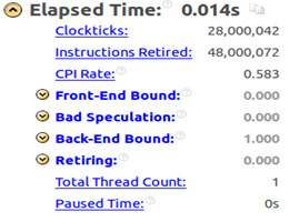
Figure 25: Intel® VTune™ Amplifier summary analysis.
Notice that the front-end bound is zero and the back-end bound is 1.0 for one thread and the exact inverse for two threads, due to the OpenMP overhead previously mentioned.
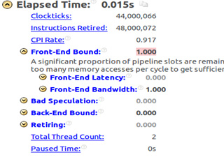
Figure 26: Intel® VTune™ Amplifier summary analysis.
Intel® Parallel Advisor Tips for Multithreading
Intel Parallel Advisor is an important tool that helps analyze the impact of parallelism before actually doing it. This tool identifies the most expensive pieces of code and estimates the speedup achieved by multithreading.
The use of Intel Parallel Advisor consists of four steps: (1) survey analysis, (2) annotation analysis, (3) suitability analysis, and (4) correctness analysis. The survey analysis shows the basic hotspots that can be candidates for parallelization. Figure 27 shows a top-down view, where the top of the figure indicates that the “transport” module is the most expensive candidate. The Intel Parallel Advisor screen exhibits information like the time spent in each function, the loop type (vector or scalar), and the instruction set (Intel AVX, Intel AVX2, Intel SSE, and so on). The same information is shown in the bottom part of the figure, but in a caller-callee tree structure. This gives a top-down view for a module’s behavior, providing information about microarchitecture issues as well as the identification of the most expensive loops that become candidates to parallelism. In this case, the main loop in the function “ktdd_rt” inside the “transport” module that takes 98 percent of total time is shown in the bottom half of the figure.
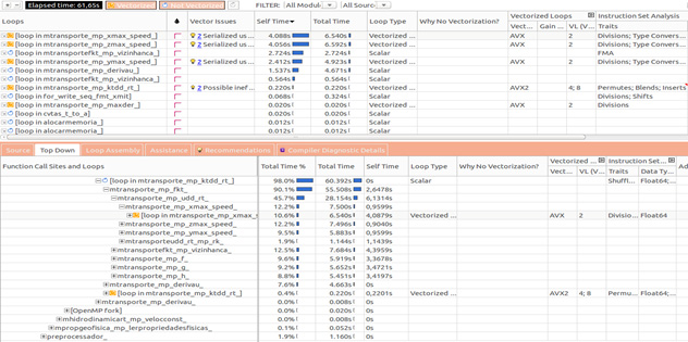
Figure 27: Intel® Parallel Advisor.
Once the loops with the most computational effort are identified, annotations are inserted in the source code9. Annotations are inserted to mark the places in the serial program where Intel Advisor should assume parallel execution and synchronization will occur. Later the program is modified to prepare it for parallel execution by replacing the annotations with parallel framework code so that parts of the program can execute in parallel. Identify parts of the loops or functions that use significant CPU time, especially those whose work can be performed independently and distributed among multiple cores. Annotations are either subroutine calls or macro uses, depending on which language you are using, so they can be processed by your current compiler. The annotations do not change the computations of the program, so the application runs normally.
The annotations that are inserted mark the proposed parallel code regions for the Intel Advisor tools to examine in detail. The three main types of annotations mark the location of:
- A parallel site. A parallel site encloses one or more tasks and defines the scope of parallel execution. When converted to a parallel code, a parallel site executes initially using a single thread.
- One or more parallel tasks within the parallel site. Each task encountered during execution of a parallel site is modeled as being possibly executed in parallel with the other tasks and the remaining code in the parallel site. When converted to parallel code, the tasks will run in parallel. That is, each instance of a task's code may run in parallel on separate cores, and the multiple instances of that task's code also runs in parallel with multiple instances of any other tasks within the same parallel site.
- Locking synchronization, where mutual exclusion of data access must occur in the parallel program.
For our flow media problem, annotations were inserted in places shown in the code sample below. The gain estimate analyses performed by Intel Parallel Advisor are shown in Figures 28 and 29. The piece of code where site and task annotations were inserted are shown below. The first site is around the function “maxder” and the second is around the loop that computes velocity field for each finite element in the mesh.
call annotate_site_begin("principal")
	call annotate_iteration_task("maxder")
	call maxder(numLadosELem,ndofV,numelReserv,vxmax,vymax,vzmax,vmax,phi,permkx,v)
call annotate_site_end

call annotate_site_begin("loop2")
	do nel=1,numel
		call annotate_iteration_task("loop_nelem")
		[…]
	end do
call annotate_site_end
The next step is to execute the suitability report to obtain an estimate of how much faster the code can run with more than one thread. Figure 28 shows the performance gain estimate for the first site annotated (“principal” loop) and it's linear until 32 threads, as can be seen in the green region of the graphics of gain versus the CPU count (threads).
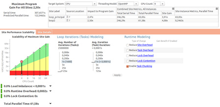
Figure 28: Intel® VTune™ Amplifier summary analysis.
Figure 29 shows that the gain is estimated to be linear until 64 threads for the second site annotated (“loop2” loop).
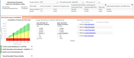
Figure 29: Intel® VTune™ Amplifier summary analysis.
At the Impact to Program Gain area on the screen, Intel Advisor suggests a gain of performance about 2.5 times faster (2.47 for the first site and 2.50 for the second site) with four OpenMP parallel threads (CPU Count set to four) in places where annotation sites were put in. This value is applicable to only these two sites. For a total estimate of the gain of performance, it's necessary to insert annotations in some more expensive loops.
Parallelization in multithread environment
In order to verify how fast the code can be executed, some tests were executed in a cluster node composed of four Intel® Xeon® processor E5-2698 v3 (40 M cache, 2.30 GHz) processors with 72 total cores, including hyper-threading.
Two different meshes were executed, 100×20×100 and 200×40×200, in order to compare how speedup varies as a function of the number of threads in each one. In the previous section an initial analysis was performed using Intel Parallel Advisor, which indicated that for the sites annotated, one can get a linear speedup at up to 32 threads and in this section one can verify whether those predictions were confirmed.
The code could be executed only until 47 threads without any kind of problem. At greater values, a segmentation fault occurs. The reason for this problem is left for further investigation.
For the first mesh (100×20×100) a linear speedup was observed in Figure 30, only until 25 threads where this speedup decreases and varies linearly again until 32, with the same value for 25 threads. For more than 32 threads, the speedup increases again but above a linear rate. This result shows there are three different ranges where gain of performance increases: (1) from 1 to 25, (2) from 26 to 32, and (3) from 33 to 47. This apparently strange behavior can be possibly caused by two events: the hyper-threading and the so called “numa-effect.”
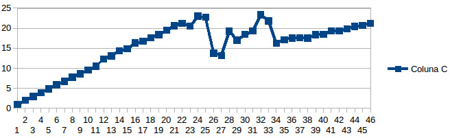
Figure 30: Speedup x number of threads.
As mentioned in10, Non Uniform Memory Access (NUMA) is a solution to scalability issues in SMP architecture and also a bottleneck for performance due to memory access issues.
“As a remedy to the scalability issues of SMP, the NUMA architecture uses a distributed memory design. In a NUMA platform, each processor has access to all available memory, as in an SMP platform. However, each processor is directly connected to a portion of the available physical memory.
In order to access other parts of the physical memory, it needs to use a fast interconnection link. Accessing the directly connected physical memory is faster than accessing the remote memory. Therefore, the OS and applications must be written having in mind this specific behavior that affects performance.”
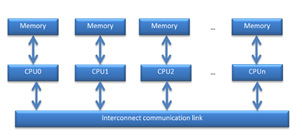
Figure 31: Typical NUNA architecture.
Since the cluster node is composed of four CPUs (multi-socket system), as shown in Figure 31, which one connected at its particular cache memory, NUMA effect can occur as a consequence.
As shown in Figure 32, Intel® Hyper-Threading Technology permits one physical core to execute two simultaneous threads by the use of a pair of registers sets. When a thread executes an operation that lets the execution unit be idle, the second thread is put to run, increasing CPU throughput (see Figure 33). However, there is only one physical core and the gain of performance will not be double for a high CPU bound application.
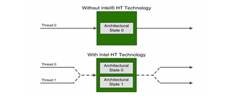
Figure 32: Intel® Hyper-Threading Technology.
As explained in11, “In the diagram below, we see an example of how processing performance can be improved with Intel HT Technology. Each 64-bit Intel Xeon processor includes four execution units per core. With Intel HT Technology disabled, the core’s execution can only work on instructions from Thread 1 or from Thread 2. As expected, during many of the clock cycles, some execution units are idle. With Hyper-Threading enabled, the execution units can process instructions from both Thread 1 and Thread 2 simultaneously. In this example, hyper-threading reduces the required number of clock cycles from 10 to 7.”
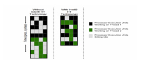
Figure 33: Intel® Hyper-Threading Technology.
This reduction from 10 to 7 clock cycles represents a gain of performance up to 1.5 times faster, not more than that, for this particular example.
Figure 34 shows the graphics for the second mesh (200×40×400) that executes 1281 transport steps and is 1000 times bigger than the previous (100×20×1000) mesh, so it's a high and more critical CPU bound task. Results show that linear speedup is achieved only until 16 threads.
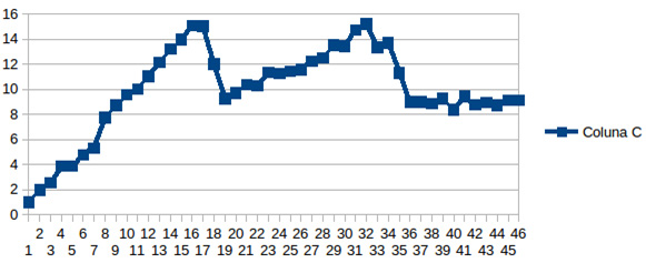
Figure 34: Second mesh.
As in the previous mesh, this one presents a pattern of three different ranges where speedup has a particular behavior. Region one presents a linear gain (1 to 16 threads) as does the second one (19 to 32 threads). The third region presents almost no gain.
Regardless of the differences in execution time between the two tests, the similarities are important to point out, because they indicate that the causes for not obtaining linear speedup from 1 to 36 threads as predicted by Intel Parallel Advisor are the same: the NUMA effect and hyper-threading.
Tables 3 and 4 show the execution time as a function of the number of threads.
Table 3: Threads × time in seconds - 100×20×100.
Table 4: Threads × time in seconds - 200×40×200.
In order to achieve a better gain, other tests can be performed with a higher workload. Amdahl's Law12 affirms that the speedup possible from parallelizing one part of a program is limited by the portion of the program that still runs serially, which means that despite the number of parallel regions in the program and the number of threads, the total gain is bound by the serial portion of the program. In this case, for the tests presented further, the total number of transport steps is increased via a diminishing Courant number (Cr) (from 0.125 to 0.0125), keeping the total simulation final time equal to 0.8 days, just like all the previous tests. For the 100x20×100 mesh, the number of transport steps increased from 641 to 6410 and for the 200×40×200 mesh, the number increased from 1281 to 12801. For both meshes the amount of work was 10 times the previous ones, because the Cr was also diminished by a factor of 10.
Figure 35 shows speedup for the mesh 100x20x100 with Cr = 0.0125, where one can notice that the gain increases practically linearly until 34 threads, which corresponds to the number of physical cores in the cluster node, since it has 4 processors with 9 cores each and hyper-threading. As the previous test showed in Figure 30, hyper-threading was not efficient enough to achieve more gain. Nevertheless, as opposed to the previous test, this one presented a gain near to linear until the number of threads matched the number of physical cores. This result indicates that for a higher workload, the code benefits from multicore architecture, but one question still remains: Even though the test with the 200×40×200 mesh (Figure 34) has a higher workload, the speedup is good only until 16 threads, no more than that. What kind of work can be augmented such that a gain appears?
Basically, it's possible to increase workload by two different ways: (1) a more dense mesh, which has more points and therefore more finite elements inside a particular region and (2) more transport steps that can be caused by two different factors: a higher simulation total final time and a lower CR. The test shown in Figure 35 was performed only with additional time steps; the total elapsed time (total wallclock time) for one thread was 403,16 seconds and for 36 threads was 14,22 seconds which is about 28 times faster.
The other approach, which consists of increasing both the number of transport steps and the mesh density, is presented in Figure 36 where the total time for one thread is 6577,53 seconds and for 36 threads is 216,16 seconds, leading to a speed-up about 30 times faster. With these two ways of augmenting the workload, the gain still remained almost linear for the number of physical cores, indicating that the factor that helps parallelism to achieve a good speed-up is the increase of time steps and not the mesh density.
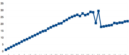
Figure 35: Mesh 100×20×100 with Cr = 0.0125.
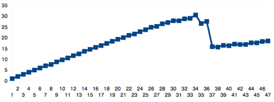
Figure 36: Mesh 200×40×40 with Cr = 0.0125.
Table 5 compares both strategies for increasing workload and whether the gain is linear (good or bad speedup).
|
|
100×20×100 mesh |
200×40×200 mesh |
|---|---|---|
| Cr = 0.125 | Bad speedup | Bad speedup |
| Cr = 0.0125 | Good speedup | Good speedup |
Table 5: Meshes x Different Courant Numbers.
Table 5 suggests that the factor that contributes to a good gain is the increase in total transport steps and not the mesh density. The execution with more transport steps decreases the percentage of time spent accessing the cache memory of other sockets, therefore reducing the NUMA effect. This result indicates which cases will probably benefit from many core processor architecture such as the Intel® Xeon Phi™ coprocessor.
Conclusion and Future Work
This paper presented an analysis of the gain in performance through the use of auto-vectorization provided by the compiler and also showed where the most impacted bottlenecks in the code are to vectorize and improve performance even more. Memory bound seems to be the cause of back-end bound, creating some difficulties for achieving the optimization goal. To accomplish that, some changes should be made in data structures and in the code that accesses them. Compiler reports are considered for analyzing the reasons that some parts of code could not be vectorized automatically. Identifying those reasons is a crucial point to permit more improvements. The application was tested with different sizes of problems to compare the speedup behavior. It was clear that auto-vectorization reduced execution time by a factor of 2.5 for small cases and by higher than 3.0 for bigger cases.
For future steps in this project, semi-auto vectorization should be studied and a refactoring in the code may be necessary to simplify the manipulation of data structures and vectorization of the loops the compiler could not vectorize by itself. To amplify the test cases, bigger meshes have to be used to investigate how faster it’s possible to achieve for real problems.
Another important issue considered in this paper is the multi-thread (OpenMP) approach that showed that with two threads a speedup of 1.8 times faster can be achieved despite the issues still to be considered. Analysis with Intel Advisor indicated that the potential speedup is about 32, but tests performed in a cluster node showed that a linear gain was achieved only for 25 or 16 threads. This difference between what Intel Advisor predicted and what actually executed is suspected of being caused by the NUMA effect and hyper-threading. Tests increasing the workload in time instead of in space minimized this problem by reducing the percentage of time spent accessing the cache memory of other sockets, therefore reducing the NUMA effect and linear speedup for the number of physical cores should be accomplished.
References
1 “How to Tune Applications Using a Top-Down Characterization of Microarchitectural Issues.” Intel® Developer Zone, 2016.
2 Correa, M. R. and Borges, M. R., “A semi-discrete central scheme for scalar hyperbolic conservation laws with heterogeneous storage coefficient and its applications to porous media flow.” International Journal for Numerical Methods in Fluids. Wiley Online Library. 2013.
3 “Intel Architecture Instruction Set Extensions Programming References.” Intel® Developer Zone, 2012.
4 “Fortran Array Data and Arguments and Vectorization.” Intel® Developer Zone, 2012.
5 “A Guide to Vectorization with Intel Compilers,” Intel® Developer Zone, 2012.
6 “Introduction to Intel Vector Advanced Vector Extensions.” Intel® Developer Zone, 2011.
7 “Clockticks per Instructions Retired.” Intel® Developer Zone, 2012
8 Optimization Manual
9 About Annotations (https://software.intel.com/en-us/node/432316)
10 NUMA effects on multicore, multi socket systems (https://static.ph.ed.ac.uk/dissertations/hpc-msc/2010-2011/IakovosPanourgias.pdf)
11 https://www.dasher.com/will-hyper-threading-improve-processing-performance/
12 https://software.intel.com/en-us/node/527426