Overview
The ability to understand people and their emotional states through spoken language is a skill that many people take for granted. Speech is among the most natural ways to express emotions. Expressing emotions is important in text messaging and emails where emojis are often used to represent associated emotions.
A speech emotion recognition (SER) system is a collection of methodologies that process and classify speech signals to detect emotions embedded in them. Such a system can be used in a variety of application areas, like interactive voice-based assistants, caller-agent conversation analysis, or psychological tests.
This tutorial examines how to detect underlying emotions in recorded speech samples by analyzing the acoustic features of the speech using a classification model of emotion elicited by audio based on deep neural networks, specifically convolutional neural networks (CNN).
The proposed system uses the following suite of frameworks that are included with AI Tools to improve the overall performance of feature extraction and model training process:
- Intel® Distribution of Python* takes advantage of the most popular and fastest growing programming language with underlying instruction sets optimized for Intel® architectures. This helps to achieve near-native performance through accelerating core Python numerical and scientific packages that are built using Intel® Performance Libraries.
- Intel® Extension for Scikit-learn* accelerates the scikit-learn applications for dimensionality reduction techniques like Principal Component Analysis (PCA).
- Intel® Extension for TensorFlow* provides an added performance boost on Intel hardware that takes advantage of up-to-date features and optimizations including Intel® Advanced Vector Extensions 512 (Intel® AVX-512) and Intel® Advanced Matrix Extensions (Intel® AMX).
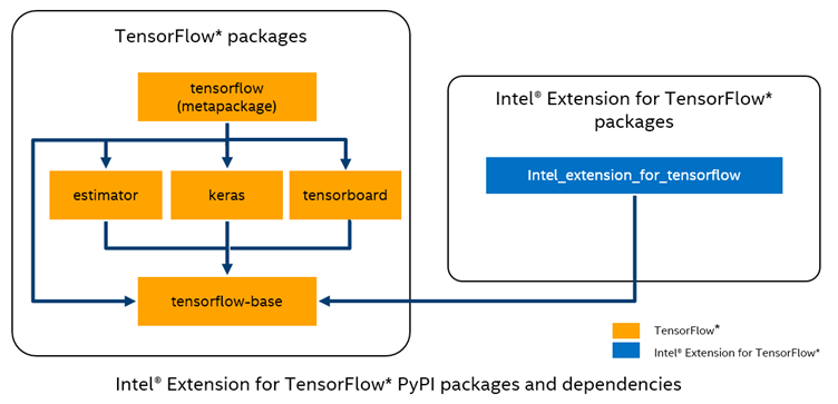
Figure 1. Intel Extension for TensorFlow packages and dependencies
Prerequisites
Hardware Requirements
|
Item |
Details |
|---|---|
|
Architecture |
x86_64 |
|
CPU Op-modes |
32 bit, 64 bit |
|
Byte Order |
Little endian |
|
Address Sizes |
46 bits physical, 48 bits |
|
Virtual CPUs |
24 |
|
Online CPU List |
0-23 |
|
Threads per Core |
2 |
|
Cores per Socket |
6 |
|
Sockets |
2 |
|
Non-Uniform Memory Access (NUMA) Nodes |
2 |
|
Vendor ID |
Genuine Intel |
|
CPU Family |
6 |
|
Model |
85 |
|
Model Name |
Intel® Xeon® Gold 6128 processor at 3.40 GHz |
Software Requirements
| Library | Version |
|---|---|
| Python | 3.9.15 Intel Corporation |
| TensorFlow | 2.9.1 |
| Librosa | 0.9.2 |
| NumPy | 1.23.5 |
| scikit-learn | 1.2.0 |
| SciPy | 1.8.1 |
| Matplotlib | 3.6.2 |
Code Snippets
The Jupyter* Notebooks used for this article can be found in Code.zip. All of the notebooks are designed to run on Intel® Developer Cloud in a JupyterLab environment. For more information, see Implementation in a Local conda* Environment and Implementation in Intel Developer Cloud.
Four notebook files are in the compressed archive:
Combining_Dataset.ipynb
Helps to automate the download process of getting the dataset. Some manual intervention is required, which is explained in this notebook. It also has the code to combine two downloaded datasets to form the dataset that is used to train the model.
Feature_Extraction.ipynb
Contains the code to extract the features required for training .csv files: train_features.csv and test_features.csv. These files are included in the Code.zip folder. You can use these two .csv files directly and run the Proposed_System.ipynb notebook (explained next) without extracting features and combining dataset steps.
Proposed_System.ipynb
Contains the actual training code that reads the .csv files, does model training, and evaluates performance matrices.
Baselines.ipynb
Contains the code for the baseline traditional classifiers used in this article. This includes feature extraction, hyperparameter tuning (using Optuna* framework), along with the performance metric evaluations. This notebook is extremely time and compute intensive, and can take several hours to complete.
To access these .ipynb files and .csv files, you must import them to Intel Developer Cloud:
- Open a Jupyter Notebook.
- Upload the .zip file to Intel Developer Cloud, and then unzip the folder.
Create an Intel-Optimized Python* Environment
Implementation in a Local conda* Environment
The environment to run this code can be created in any Python with conda environment by running each of the following commands:
# Create a new environment with intelpython_full package
 conda create -n <env name> intelpython3_full


#Activate the newly created environment
 conda activate <env name>


# Install Intel AI Kit for Tensorflow
 conda install intel-aikit-tensorflow


# Install/Upgrade additional packages
 pip install ipykernel pandas matplotlib plotly glob tqdm lightgbm optuna seaborn
 pip install --upgrade numpy


# Install the Python audio processing library
 pip install --user librosa --force-reinstall


# Creating a IPython kernel using the new conda environment
 python -m ipykernel install --user --name=<env_name>


# Run Jupyter Notebook
 jupyter notebook
After you run the commands, activate the new IPython kernel <env_name> that you created in your Jupyter Notebook and use it to run the notebook.
Implementation in Intel® Developer Cloud
To create a new account and set up a new Intel-optimized Python environment:
- Go to the Get Started page, and then select Get Free Access.
- Sign in to your Intel Developer Cloud account.
- To start using JupyterLab on Intel Developer Cloud, do one of the following:
- Navigate to JupyterLab.
- Navigate to Get Started. At the bottom of the page, select Launch JupyterLab.
- To launch a new terminal window, select the Launcher tab, and then select Terminal.
Intel Developer Cloud comes installed with conda environments that contain the necessary Intel-optimized packages for frameworks, like TensorFlow and PyTorch*. Since the proposed system uses TensorFlow, the predefined TensorFlow environment is cloned to create a new environment locally and to install the additional packages that are required to run the code.
To run the code, run each of the following commands:
# Cloning the existing Intel AI Analytics Toolkit TensorFlow environment

conda create --name <env_name> --clone tensorflow


# Activating the new virtual environment

source activate <env_name>


# Installing Python Audio Processing Library LibROSA


# Upgrading NumPy to latest version to avoid conflicts with LibROSA

pip install --user --upgrade numpy

# Installing LibROSA

pip install --user librosa --force-reinstall


#Checking whether LibROSA is installed correctly

python -c 'import librosa; print(librosa.__version__)'


# Installing additional packages

pip install --user plotly optuna lightgbm


# Creating a IPython kernel using the newly created conda environment

python -m ipykernel install --user --name=<env_name>
The new environment is now ready and can be used to run the notebooks in the Code.zip file. In your Jupyter environment, make sure that the selected IPython kernel is <env_name>.
Solution Design
Datasets
The datasets used in this work are RAVDESS and TESS. These datasets are available to download and provide good inter-rater reliability that's based on the observation that including two datasets made the model more generalized and less correlated to the content that is conveyed in the audio samples. Including two datasets has also improved the support provided to each emotional class from the dataset.
RAVDESS
The RAVDESS dataset contains 2,452 recordings (60 speech, 44 singing) of 24 actors (12 male, 12 female). This system only uses the audio-only modality for analysis. Actors vocalised two distinct statements in the speech and song conditions. The two statements were each spoken with eight emotional intentions (neutral, calm, happy, sad, angry, fearful, surprise, and disgust), and sung with six emotional intentions (neutral, calm, happy, sad, angry, and fearful). All emotional conditions except neutral were vocalized at two levels of emotional intensity, normal and strong. Actors repeated each vocalization twice.
TESS
The TESS dataset contains a set of 200 target words that two actresses spoke in the carrier phrase “Say the word _____.” Recordings were made of the set portraying each of seven emotions (anger, disgust, fear, happiness, pleasant, surprise, sadness, and neutral). The dataset includes 2,800 responses to stimuli.
Combining RAVDESS and TESS Datasets (TESS Pipeline)
For this task, the dataset is built using 5,252 samples from:
- Ryerson Audio-Visual Database of Emotional Speech and Song (RAVDESS)
- Toronto Emotional Speech Set (TESS)
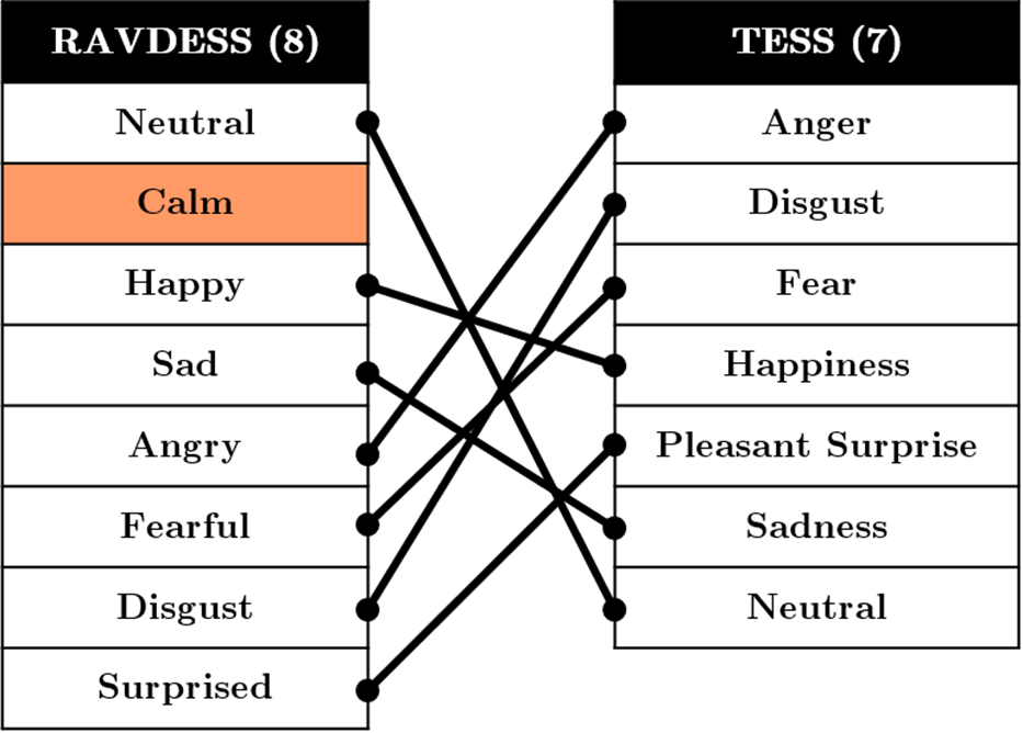
Figure 2.
The classes the model predicts are:
- 0 = neutral
- 1 = calm
- 2 = happy
- 3 = sad
- 4 = angry
- 5 = fearful
- 6 = disgust
- 7 = surprised
The audio samples are split into 16 gender-based classes.
The emotion mapping is done as illustrated in Figure 2. The TESS dataset does not contain the emotion “Calm” so therefore does not have a mapping.
The distribution of the combined dataset with support provided by each emotion class and dataset is in Figure 3:
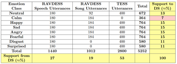
Figure 3.
Implement Datasets on Intel Developer Cloud
Implement datasets in Intel Developer Cloud using the notebook Combining_Datasets.ipynb.
To download and combine the datasets:
- Download the RAVDESS dataset:
- Go to RAVDESS.
- Download Audio_Song_Actors_01-24.zip and Audio_Speech_Actors01-24.zip.
- Create a directory called DATASET, and then extract the contents of both files to that directory.
- In the DATASET directory for TESS dataset, create two directories: Actor_26 and Actor_28.
- Download the TESS dataset file: dataverse_files.zip.
Note This download requires manual steps and license acceptance.
- Navigate to Intel Developer Cloud, and then upload dataverse_files.zip.
- Create a new directory called TESS_Toronto_emotional_speech_set_data, and then extract the contents of dataverse_files.zip to it.
- Run the TESS pipeline that combines the TESS dataset into the RAVDESS dataset.
- Since the classes are contained in the filename of the audio samples, remove the directory structure of the DATASET folder. A directory containing 52,52 audio .wav samples appears.
Audio Feature Extraction
The proposed system uses multiple discrete energy-based audio features such as MFCC, Mel Scale, and chroma, which are extracted from the audio files. This is because emotion is correlated to energy features, not other audio features. MFCC feature extraction contributes 40 features, Mel Scale features extraction contributes 128 features, and chroma features extraction contributes 12 features amounting to a total of 180 features being extracted from a single audio file. A brief idea regarding these features is as follows:
Mel Spectrograms
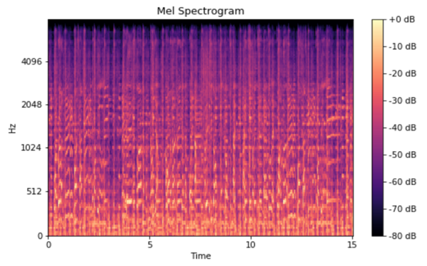
Figure 4.
Studies have shown that humans do not perceive frequencies on a linear scale. We are better at detecting differences in lower frequencies than higher frequencies. For example, we can easily tell the difference between 500 and 1000 Hz, but we can hardly tell the difference between 10,000 and 10,500 Hz, even though the distance between the two pairs is the same. In 1937, Stevens, Volkmann, and Newmann proposed a unit of pitch, called the mel scale, where equal distances in pitch sounded equally distant to the listener. A mel spectrogram converts the frequencies to the mel scale. For more information, see References.
# Code to extract Mel Features from an audio sample

import librosa

import numpy as np

x, sample_rate = librosa.load(“<audio_filename>.wav”)

mels = np.mean(librosa.feature.melspectrogram(x, sr=sample_rate).T,axis=0)
MFCC Spectrograms
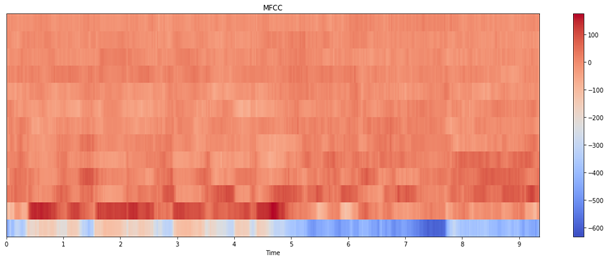
Figure 5.
MFCCs are coefficients that collectively make up a mel-frequency cepstrum (MFC). MFC is a representation of the short-term power spectrum of a sound that's based on a linear cosine transform of a log power spectrum on a nonlinear mel scale of frequency. They are derived from a type of cepstral representation of the audio clip (a nonlinear spectrum-of-a-spectrum). In MFC, the frequency bands are equally spaced on the mel scale, which approximates the human auditory system's response more closely than the linearly spaced frequency bands used in the normal cepstrum. This frequency warping can allow for better representation of sound.
# Code to extract MFCC Features from an audio sample

import librosa

import numpy as np

x, sample_rate = librosa.load(“<audio_filename>.wav”)

mfccs = np.mean(librosa.feature.mfcc(y=x, sr=sample_rate, n_mfcc=40).T, axis=0)
Chroma Spectrograms
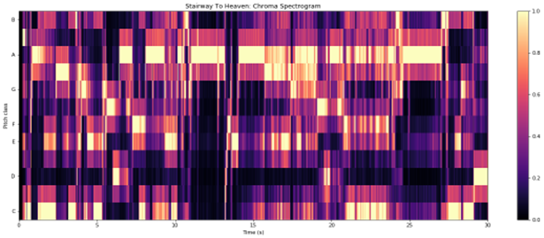
Figure 6.
The term chroma feature (or chromogram) closely relates to the twelve different pitch classes. Chroma-based features, which are also referred to as a pitch class profile, are a powerful tool for analyzing music whose pitches can be meaningfully categorized and whose tuning approximates to the equal-tempered scale. One main property of chroma features is that they capture harmonic and melodic characteristics of music, while being robust to changes in timbre and instrumentation. Assuming the equal-tempered scale, one considers twelve chroma values represented by the set {C, C#, D, D#, E, F, F#, G, G#, A, A#, B} that consists of the twelve-pitch spelling attributes as used in Western music notation.
# Code to extract Chroma Features from an audio sample

import librosa

import numpy as np

x, sample_rate = librosa.load(“<audio_filename>.wav”)

stft = np.abs(librosa.stft(x))

chroma = np.mean(librosa.feature.chroma_stft(S=stft, sr=sample_rate).T,axis=0)
Implement Audio Feature Extraction on Intel Developer Cloud
Implement these steps in Intel Developer Cloud using the notebook Feature_Extraction.ipynb.
Important You must do these steps after running the steps in Implement Datasets on Intel Developer Cloud.
To extract the audio feature:
- Create a function that reads the files from the DATASET directory, and then extract the gender and emotion files.
- Create a label for the files in the dataset that follows the format gender_emotion (for example, male_angry or female_happy).
- Split the dataset into train (80%) and test data (20%).
- Extract three types of the following features from each of the audio samples using the built-in functions of the Python audio processing library LibROSA:
- MFCC (librosa.feature.mfcc): 40 features
- Chroma (librosa.chroma_stft): 12 features
- Mel Features (mean of librosa.feature.melspectrogram): 128 features
- Combine the 180 features of the train and test datasets, and the save the features to the files train_features.csv and test_features.csv, respectively.
Reduce a Feature Set Dimensionality Using PCA
The proposed system reduces the number of features at the same time attempting to keep as much information as possible using a technique of dimensional reduction called PCA. This helps reduce the number of features to 78 while capturing 95% of the variance of the original feature set.
Baseline Classifiers Models
To establish a baseline for comparison, the proposed system results were compared to results from traditional machine learning classifiers. After using the Optuna* framework for hyperparameter tuning, the following traditional classifiers were compared:
- Simple Models: KNN, LR, DT
- Ensemble Models: Bagging (RF), Boosting (XGB, LGBM)
- Artificial Neural Network Model: MLP
- Soft Voting Classifier Ensemble Models: A combination of the best performing classifiers grouped using soft voting.
- V1: MLP, KNN
- V2: KNN, XGB, MLP
- V3: XGB, MLP, RF, LR
- V4: MLP, XGB
Implement Baseline Classifiers on Intel Developer Cloud
The notebook Baselines.ipynb has the implementation steps for baseline classifiers that include hyperparameter tuning on Intel Developer Cloud.
- The notebook compares a lot of classifiers. Hyperparameter tuning for each of these classifiers is an extremely CPU-intensive task and can take multiple hours and runs to complete.
- If it is not required, do not run hyperparameter tuning. The best of the parameters have already been collected and are assigned as parameters for these classifiers.
- Only run the hyperparameter tuning if there is a change to the dataset or the overall structure of the program or features used to train the model changes.
Proposed System Architecture
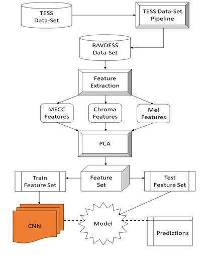
Figure 7.
After experimenting with multiple combinations of numbers and sizes for convolution layers, FC layers, optimizers, batch sizes and epochs to get the best performance, the final CNN was designed as follows:

Figure 8.
The convolution layers work to extract high-level complex features from the input data while the FC layers learn nonlinear combinations of these features to be used for classification. To avoid over-fitting, and more aggressive dropouts, L1 and L2 regularization and batch normalization at various convolution and FC layers were applied.
Implementation in Intel Developer Cloud
The implementation steps are in the notebook Proposed_System.ipynb and are performed on Intel Developer Cloud.
The following steps are performed in the proposed system:
- The train_features.csv and test_features.csv files are read and converted into a data frame.
- PCA is performed in the data frame to reduce the number of features to 78 while capturing 95% of the variance of the original feature set.
- The captured 78 features are passed to the proposed CNN model to train and test the model.
- The model is trained for 30 epochs. It stops early if validation accuracy is consistent for 20 iterations.
- The model is saved as an h5 file and the classification report, confusion matrix, accuracy, and loss graphs display.
Verbose Messages
If the code you are running is using Intel-optimized libraries and frameworks, you can see verbose messages while importing libraries or frameworks. For example:
![]()
Figure 9.
The environment that you set up uses Intel Extension for Scikit-learn to optimize a scikit-learn package for better performance.
![]()
Figure 10.
The TensorFlow that is used in the environment uses Single Instruction Multiple Instruction (SIMD), which is a type of parallel processing used to improve performance. The TensorFlow that you set up in the environment is designed to use oneAPI Deep Neural Network Library (oneDNN). The library provides highly optimized implementations of deep learning building blocks using Intel® Advanced Vector Extensions 2, Intel AVX-512, and FMA (Fused Multiply-Add) SIMD instructions to improve its performance. The SIMD instructions used by TensorFlow may vary depending upon the hardware used to perform deep learning training and inference.
Results
The proposed system performed better than the baseline classifiers by reaching an accuracy of 87%, which makes it one of the best performing SER systems that uses a single modality for emotion prediction across multiple datasets. From the results, it is evident that splitting the data into gender classes resulted in a better model. It is also observed that using multiple features together (such as MFCC, chromas, and mels) results in a more robust model compared to a model that uses a single feature. The process of dimensional reduction using PCA helped significantly to improve the accuracy of the model.
Classification Report
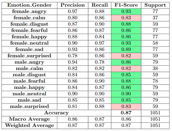
Figure 11.
Confusion Matrix
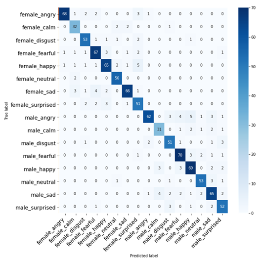
Figure 12.
Accuracy and Loss Graphs

Figure 13.
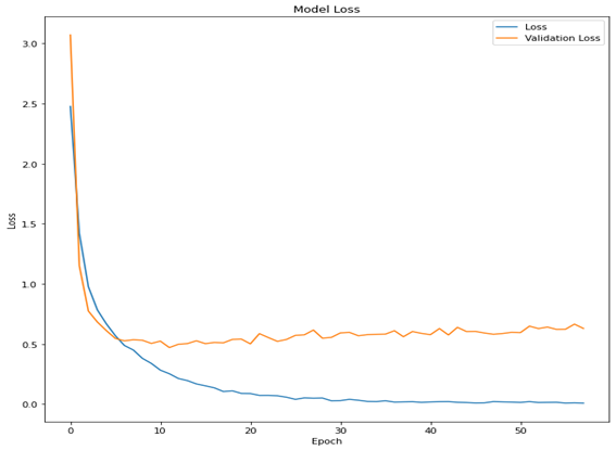
Figure 14.
Comparison with Baseline Classifiers
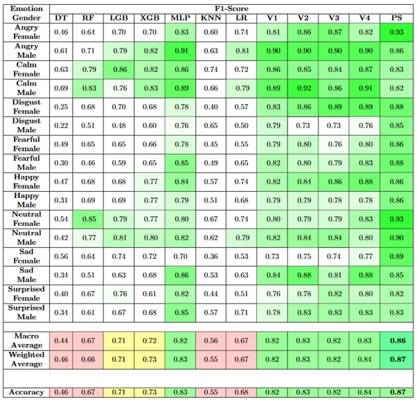
Figure 15.
In the previous table, it is clear that the variation of the emotions across classes was significantly reduced and the classification performance improved. Out of the classifiers implemented, the best-performing classifiers were XGB and MLP. As a result of combining them using equally weighted soft voting, the resultant classifier V4 achieved an overall F1-score of 84% but exhibited lower F1-scores for certain emotional gender classes like Disgust Male, Happy Male, and Sad Female.
In the proposed system, the overall accuracy has improved to 87% and the F1-scores have also become more balanced across the emotional gender classes as compared to the baseline classifiers, which makes this approach a good methodology for emotional classification.
Performance Comparisons
import os
# Intel Extension for TensorFlow Optimizations
os.environ['TF_ENABLE_ONEDNN_OPT'] = "1"

os.environ[TF_ENABLE_MKL_NATIVE_FORMAT'] = "1"
# KMP Optimizations
os.environ['KMP_BLOCKTIME'] = "0"

os.environ['KMP_AFFINITY'] = "granularity=fine,compact,1,0"

os.environ['KMP_SETTINGS'] = "1"
# OMP Optimizations
os.environ['OMP_NUM_THREADS'] = "12"
# Intel Extension for Scikit-learn Optimizations
from sklearnex import patch_sklearn

patch_sklearn()
# TensorFlow Optimizations
import tensorflow

tensorflow.config.threading.set_intra_op_parallelism_threads(12)

tensorflow.config.threading.set_inter_op_parallelism_threads(2)

tensorflow.config.set_soft_device_placement(True)
|
|
Unoptimized |
Intel-Optimized |
Optimization Factor |
|---|---|---|---|
|
Total Training Time |
1787 seconds/run |
1118 seconds/run |
1.6x |
|
Average Time/Epoch |
51 seconds/epoch |
32 seconds/epoch |
1.6x |
Conclusion and Future Work
This article gives a detailed analysis of an efficient SER system that uses multiple datasets to recognize and classify emotion using pure audio signals. In this work, an architecture based on deep neural networks was proposed to classify emotions which achieved an F1-score of 0.93 for the best and 0.82 for the worst classes. To obtain such results, feature extraction was performed to extract multiple features from the dataset along with dimensional reduction in order to filter out nonsignificant features. Overall, the proposed system was able to achieve an accuracy of 87% for the test set.
Using Intel-optimized frameworks and libraries improved the training time by 1.6x when compared to third-party libraries with minimal code changes. This reduction of training time when using Intel-optimized libraries or frameworks while maintaining the evaluation metrics of the model is extremely helpful in reducing costs and complete use of the compute resources.
The good results suggest that approaches based on deep neural networks are an excellent basis for solving SER tasks. In particular, they are general enough to work in a real-world application context correctly. Since the results can only be considered as a starting point for further extensions, modification and improvements of the proposed approach can result in even better and robust models.
References
- "Audio Emotion Classification from Multiple Datasets."
- B. P. Bogert, J. R. Healy, and J. W Tukey. "The Quefrency Analysis of Time Series for Echoes: Cepstrum, Pseudo-Autocovariance, Cross-Cepstrum and Saphe Cracking," 209–43, Proceedings of the Symposium on Time Series Analysis, 1963.
- Badshah, Abdul Malik, Jamil Ahmad, Nasir Rahim, and Sung Wook Baik. “Speech Emotion Recognition from Spectrograms with Deep Convolutional Neural Network,” 1–5, 2017 International Conference on Platform Technology and Service (PlatCon), 2017.
- Deshmukh, G., A. Gaonkar, G. Golwalkar, and S. Kulkarni. “Speech Based Emotion Recognition Using Machine Learning,” 812–817, 2019 3rd International Conference on Computing Methodologies and Communication (ICCMC), 2019.
- Pinto, M. G. de, M. Polignano, P. Lops, and G. Semeraro. “Emotions Understanding Model from Spoken Language Using Deep Neural Networks and Mel-Frequency Cepstral Coefficients,” 1–5. 2020 IEEE Conference on Evolving and Adaptive Intelligent Systems (EAIS), 2020.
- Stevens, S. S., J. Volkmann, and E. B. Newman. “A Scale for the Measurement of the Psychological Magnitude Pitch,” 185–190. The Journal of the Acoustical Society of America 8 (3), 1937.